3 Summary Statistics in Excel 3.3 Understanding Proportions 3.5 How Spread Out is the Quantitative Data?

3.4 Where’s the Center of Quantitative Data?

Goals:

\bullet

Learn to create a histogram from a frequency distribution;

\bullet

Know the different measurements of center: Mean, Median, and Mode;

\bullet

Know how each of the different measurements of center are affected

\bullet

by perturbations in data.

The reason for studying data is to gather information. Typically, we first try to summarize what the data is telling us. There are several ways of summarizing data. In this section, we will study study the summary statistics that measure the location of what one would call the center of the data.

3.4.1 Measures of Center

The Mean

The most common measurement of center of data is called the mean.

Definition (Mean).

Given a sample of $n$ data values, $x_{1},x_{2},\ldots,x_{n}$ , the sample mean, denoted by $\bar{x}$ (or sometimes called the sample average) is

\bar{x}=\dfrac{x_{1}+x_{2}+\cdots+x_{n}}{n}=\dfrac{1}{n}\sum\limits_{i=1}^{n}x% _{i}.

If our data set consists of the whole population, we calculate the mean in the same manner and denote the population mean by the Greek letter $\mu$ .

So what does the mean really tell us? The best way to explain the mean is to picture a teeter-totter with our data arranged from lowest to highest on it. The mean is the location of the fulcrum, i.e., the location where the data would balance. Let’s see some examples involving the calculation of the mean.

Example 3.4.1.

Assuming your population consists of all the numbers within the range $[0,60]$ .

(a)

Let’s predict the population mean, $\mu$ , of the data.

Since the mean acts as the balancing location of the data, we an predict that the mean of the range of values $[0,60]$ would be $\mu=30$ .
(b)

Let’s construct a random sample of 10 data values from the population. Can you determine what is $\bar{x}$ ?

Using $\tt{\color{red}\colorlet{pgfstrokecolor}{.}=RAND()}$ , we can create a random sample of values between $[0,60]$ . Recall that $\tt{\color{red}\colorlet{pgfstrokecolor}{.}=RAND()}$ only generates a random number between $[0,1]$ . Algebraically manipulating the command, we have

$\tt{\color{red}\colorlet{pgfstrokecolor}{.}=60*RAND()}.$

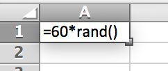
Enter this command on a new sheet in Excel within cell $\tt{\color{red}\colorlet{pgfstrokecolor}{.}A1}$ .

Figure 3.46:

Auto-fill 9 more cells in the column just below cell $\tt{\color{red}\colorlet{pgfstrokecolor}{.}A1}$ . In cell $\tt{\color{red}\colorlet{pgfstrokecolor}{.}C1}$ type: Sample Mean:. Then, in cell $\tt{\color{red}\colorlet{pgfstrokecolor}{.}D1}$ type the expression:

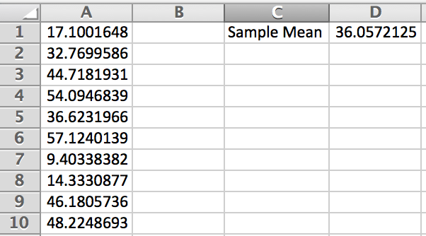
$\tt{\color{red}\colorlet{pgfstrokecolor}{.}=SUM(A1:A10)/10}$

Figure 3.47:

So in Figure 3.47, you can see that we obtained $\bar{x}=36.0572125$ . Do you obtain the same answer?
(c)

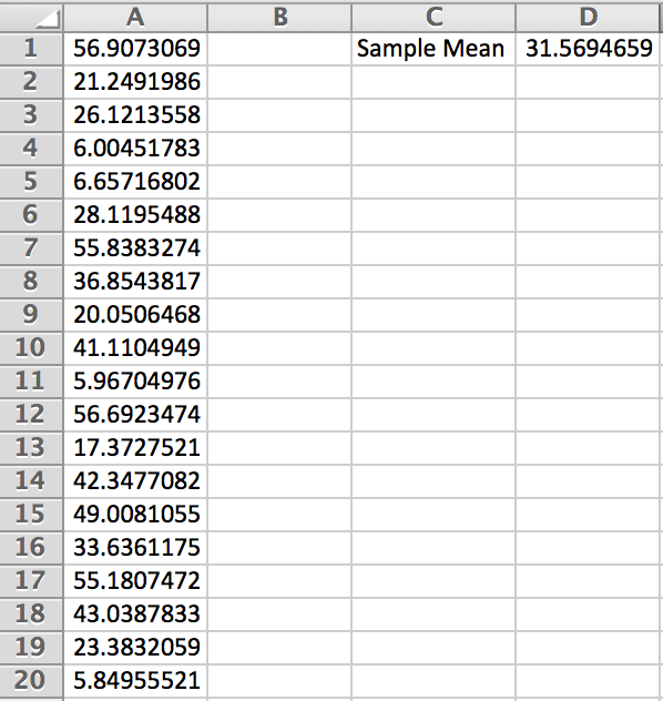
Construct a random sample of 20 data values from the population and find $\bar{x}$ . How does it relate to $\mu$ ? Auto-fill 10 more entries in the first column. Then adjust the expression in cell $\tt{\color{red}\colorlet{pgfstrokecolor}{.}D1}$ to include the new entries in column $\tt{\color{red}\colorlet{pgfstrokecolor}{.}A}$ by typing

$\tt{\color{red}\colorlet{pgfstrokecolor}{.}=SUM(A1:A20)/20}.$

Figure 3.48:

Notice that in Figure 3.48, $\bar{x}=31.5694659$ . If we were to press F9 on the keyboard, the random sample will change. Doing this, one can see that the sample means seems to be jumping round our predicted population mean. Is this a coincidence?

$\clubsuit$

In the previous example, there is no coincidence that the mean of the sample is jumping around $\mu=30$ . Ideally, we would love to know what the mean of the population, $\mu$ , is. We learned that obtaining the entire population can be rather difficult. So, $\bar{x}$ is sometimes the best we have to approximate $\mu$ .

The mean is sensitive to extreme values in the data. Going back to the teeter-totter metaphor for the mean, data values that are much much larger or much much smaller than the rest of the data will cause the mean to tend towards the extreme values. In this case, does the mean accurately portray the location of the center of the data? Let’s observe this phenomena.

Example 3.4.2.

Create a sample of data that includes nine random values between $[0,1]$ and a tenth value of 100. Compute the sample mean of the data. What do you observe happening?

On a new sheet in Excel, we have generated our data and computed the sample mean.¹¹¹¹The average is computed with the Excel command $\tt{\color{red}\colorlet{pgfstrokecolor}{.}AVERAGE(\ldots)}$ . We will encounter this command in later examples. Figure 3.49 demonstrates this.

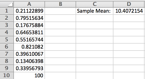
As one can see, the sample mean tends towards the value 100. However, the majority of the data is between $[0,1]$ . $\clubsuit$

In statistics, we often give the name outlier to the data value 100 as seen in the previous example.

Definition (Outlier).

A data value that tends to be an extreme in relation to other data values within the sample.

Outliers can and do happen in data. They are often the cause of outside forces such as errors in studies or rare situations. With some justification and intense analysis, some outliers can be removed from data since they can affect values such as the mean of the data.

The Median

Another common measurement of center of data is called the median.

Definition (Median).

Given a sample of $n$ data values, $x_{1},x_{2},\ldots,x_{n}$ , arranged in order from lowest to highest in value, the median is the data value that designates the location of where 50% of the data are below it. If the data set consists of an odd number of values, then the median is the middle value. If the data set consists of an even number of values, then the median is the average of the middle two values.

Example 3.4.3.

Let’s find the median of the following random samples, generated by Excel.

(a)

An odd number of data values $\ldots$

0.65 0.88 0.33

0.66 0.93 0.58

0.33 0.82 0.04

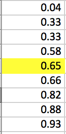
Arrange the data in order from lowest to highest by using the sort feature in Excel. Since there are an odd number of data values, then choose the middle number. In this case, the fifth data value is the median of the data. That is: $\tt{\color{red}\colorlet{pgfstrokecolor}{.}0.65}$ .

Figure 3.50:
(b)

An even number of data values $\ldots$

0.65 0.37 0.66 0.29 0.25

0.64 0.68 0.52 0.18 0.85

Arranging the data from lowest to highest by using the sort feature in Excel in cells $\tt{\color{red}\colorlet{pgfstrokecolor}{.}A1}$ through $\tt{\color{red}\colorlet{pgfstrokecolor}{.}A10}$ . Since there are an even number of values, then we need to find the two middle values of the data. In this case, the fifth and sixth data values are the middle values. We then find the average of these values to find the median of the sample.

Use the shortcut command to find the average of data values by typing:

$\tt{\color{red}\colorlet{pgfstrokecolor}{.}=AVERAGE(A5:A6)}$

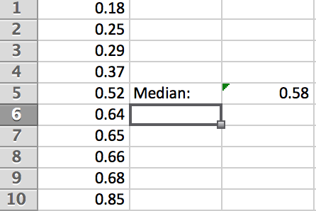
The answer to this, $\tt{\color{red}\colorlet{pgfstrokecolor}{.}0.58}$ , is the median of the sample as seen in Figure 3.51.¹²¹²As we saw with the mean, there is a shortcut for finding the median of a data set. In Excel, this involves the command $\tt{\color{red}\colorlet{pgfstrokecolor}{.}MEDIAN(\ldots)}.$

Figure 3.51:

0.65	0.88	0.33
0.66	0.93	0.58
0.33	0.82	0.04

$\clubsuit$

The median is more resistant to extreme values. If in part (b) of the previous example we replace 0.85 and replace with any value between 0.65 and larger, then the median is unaffected. However, as one can see, the median could be affected if the order of the data is changed by adding more data values or removing data values.

The Mode

Definition (Mode).

The mode of a data set is the value that occurs most often. If there is no such value, then we say that the data set has no mode.

This summary statistic is easy to recognize. But Excel will compute it rather quickly by invoking the command

\tt{\color{red}\colorlet{pgfstrokecolor}{.}MODE(\ldots)}.

Note that if $\tt{\color{red}\colorlet{pgfstrokecolor}{.}\#N/A}$ appears, it means that there is no mode.

Example 3.4.4.

Let’s generate a sample of 20 integers between $[1,3]$ and find the mode using the shortcut command.

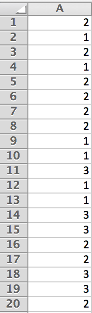
Figure 3.52 shows a sample obtained by using the $\tt{\color{red}\colorlet{pgfstrokecolor}{.}RANBETWEEN(1,3)}$ command.

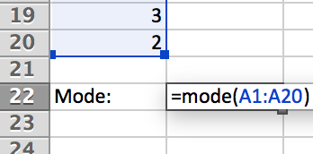
In cell $\tt{\color{red}\colorlet{pgfstrokecolor}{.}A22}$ , type Mode:. Then type the command in cell $\tt{\color{red}\colorlet{pgfstrokecolor}{.}B22}$

\tt{\color{red}\colorlet{pgfstrokecolor}{.}=MODE(A1:A20)}.

Upon hitting enter, we obtain the mode of $\tt{\color{red}\colorlet{pgfstrokecolor}{.}2}$ . $\clubsuit$

3.4.2 Symmetric and Skewed Distributions

We learned that the histogram can be used to recognize shape and patterns in the data. One particular characteristic we look for is symmetry.

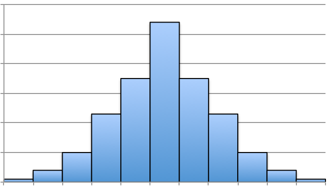
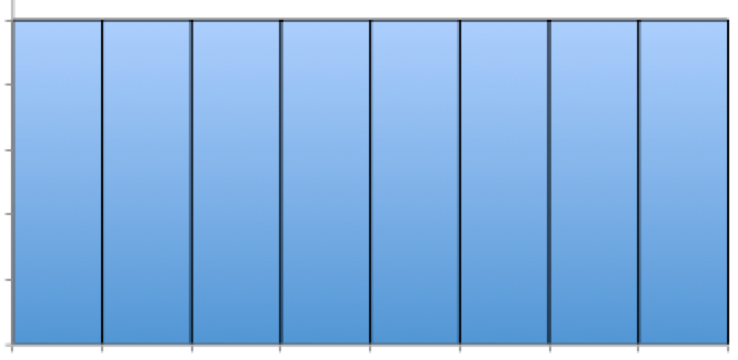
Definition (Symmetric Distribution).

Frequency distribution whose histogram exhibits similar shape to the right and left of the mean and median. For symmetric distributions, the mean and the median coincide. If there is only one mode, then it too will coincide with the mean and median.

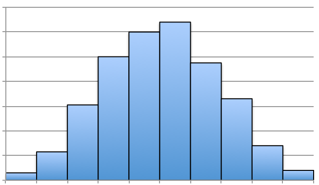
The two most familiar symmetric distributions that we will encounter look like those in Figure 3.54. In fact, the Figure a is a referred to as the bell-shaped distribution. The mean, median, and mode all coincide. This distribution will be studied further later.

Figure b seems to look rectangular. Each of the outcomes are equally likelihood to occur according to the graph. This distribution is referred to as uniform. The mean and median coincide, but there is not just one mode. Can you see why?

In reality, the samples taken will almost never exhibit a perfect symmetry. Instead, we have to use our best judgment and argue that the distribution is symmetric. For example, we saw an approximate bell-shaped image in Figure 3.26. However, one could argue that the histogram in Figure 3.26 is not symmetric and instead is skewed.

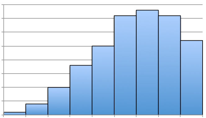
Definition (Skewed Distribution).

Frequency distribution whose histogram is non-symmetric with a fat, short-tail along with a skinny, elongated tail. Skewed Left implies the skinny, elongated tail is on the left and the mean is less than the median. Skewed Right implies the skinny, elongated tail is on the right and the mean is greater than the median.

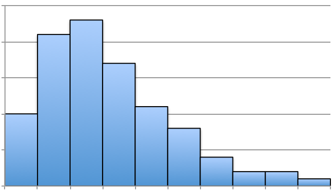
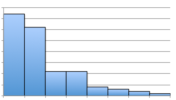
If we claim that Figure 3.26 is not symmetric, but skewed, we can see that there’s a slight, elongated left-tail. Thus, the mean is less than the median for that distribution. Below are a few additional histograms that portray skewed left, skewed right, and approximately symmetric distributions.

Concepts Check: 1. Find the mean, median, and mode of the following data: 2 3 4 2 4 1 3 2 4 3 1 2 4 4 1 4 1 3 4 2 Answer: Mean

=2.65

, Median

=3

, Mode

=4

2. Is the following histogram displaying a distribution that is skewed or symmetric?

Answer: Skewed Right

3.4.3 Exercises

1.
Answer each of the following statements as True or False.
1. (a)
  
  The average and the mean are two different calculations.
2. (b)
  
  The shortcut command for finding the mean in Excel is $\tt{\color{red}\colorlet{pgfstrokecolor}{.}MEAN(\ldots)}$ .
3. (c)
  
  The median is extremely sensitive to outliers.
4. (d)
  
  The mean and the median are not equal in a symmetric distribution.
5. (e)
  
  It is possible to have no mode.
2.
Without using the command $\tt{\color{red}\colorlet{pgfstrokecolor}{.}AVERAGE}$ , create a spreadsheet that will compute the sample mean of 7 data given. Use it to quickly compute the sample means of the following data.
1. (a)
  
  3, 2, 1, 3, 1, 3, 3
2. (b)
  
  4, 2, 1, 3, 3, 3, 4
3. (c)
  
  6.5, 12.4, 11.9, 16.7, 14.8, 6.8, 14.2
4. (d)
  
  40.4, 80.8, 43.0, 44.4, 51.2, 96.4, 53.4
3.

Using $\tt{\color{red}\colorlet{pgfstrokecolor}{.}RAND()}$ , generate a sample of 100 data values from $[60,70]$ . Compute the sample mean and median. What do you expect the population mean and median to be?
4.

Using $\tt{\color{red}\colorlet{pgfstrokecolor}{.}RANDBETWEEN()}$ , generate a sample of 100 data values from $[20,35]$ . Compute the sample mean, median, and mode. What do you expect the population mean, median and mode to be?
5.

Using $\tt{\color{red}\colorlet{pgfstrokecolor}{.}NORM.INV(RAND(),30,3.6)}$ , generate 200 data values, construct a histogram. Describe where the sample mean and median are located. Is the distribution symmetric or skewed?
6.

Perform the following: generate a random sample of 10 data values using the command $\tt{\color{red}\colorlet{pgfstrokecolor}{.}RAND()}$ . Then, calculate the sample mean, $\bar{x}$ , of the 10 data values. Store this value in a separate column. Repeat the process by generating a different set of 10 data values, and computing the sample mean, $\bar{x}$ . (Note that the new sample mean may be different.) Keep repeating this process until 30 sample means are collected. Construct a histogram of the 30 sample means collected. Describe the distribution by stating the shape, symmetry, mean, median and mode.

0.65	0.37	0.66	0.29	0.25
0.64	0.68	0.52	0.18	0.85