3 Summary Statistics in Excel 3.2 Displaying the Data 3.4 Where’s the Center of Quantitative Data?

3.3 Understanding Proportions

Goals:

\bullet

Know what proportions are and how to calculate them;

\bullet

Know the different ways of expressing a proportion;

\bullet

Understand the difference between

\hat{p}

and

p

3.3.1 Proportions

In your daily life, you may have encountered the phrase, “what is the proportion of (fill-in the blank)?” Proportions allow us to summarize what how often an attribute occurs in relation to the whole.

Definition (Proportion).

Given a sample of $n$ data values and a subset of $q$ data values from the sample having a specified attribute, the sample proportion of the specified attribute, denoted as $\hat{p}$ , is the ratio of $q$ to $n$ . That is,

\hat{p}=\dfrac{q}{n}.

If the collection of data values represents the entire population, then the proportion of the specified attribute is referred to as the population proportion of the specified attribute and is denoted as just $p$ .

Remark: It is common to express a proportion as a decimal, fraction, or a percentage. By definition, and written as a decimal, a proportion is a value ranging from 0 to 1.

Proportions are easy to calculate. By definition, we must first calculate the frequency of a specified attribute first. Frequency distributions, as a result, allow us to quickly calculated proportions. Let’s revisit an example.

Example 3.3.1.

Let’s find $\hat{p}$ for the bin $(64.1,65]$ given in the frequency distribution in Figure 3.28. The frequencies of each bin are given. All we need to do is divide the frequency for bin $(64.1,65]$ by the total number of data values in the sample, $n=100$ . Thus, $\hat{p}=3/100=0.03=3\%$ . $\clubsuit$

Example 3.3.2.

Let’s use $\tt{\color{red}\colorlet{pgfstrokecolor}{.}RANDBETWEEN(1,6)}$ , to generate a sample of 250 and calculate the sample proportion $\hat{p}$ of the value $4$ showing up.

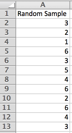
In cell $\tt{\color{red}\colorlet{pgfstrokecolor}{.}A1}$ , type RANDOM SAMPLE. Using $\tt{\color{red}\colorlet{pgfstrokecolor}{.}RANDBETWEEN(1,6)}$ , generate a random sample of 250 data points in cells $\tt{\color{red}\colorlet{pgfstrokecolor}{.}A2}$ through $\tt{\color{red}\colorlet{pgfstrokecolor}{.}A251}$ . A snapshot of our random sample is in Figure 3.44.

In cells $\tt{\color{red}\colorlet{pgfstrokecolor}{.}D1}$ through $\tt{\color{red}\colorlet{pgfstrokecolor}{.}F1}$ , copy the setup as it is in Figure 3.45.

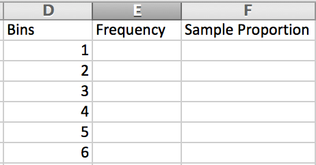
Calculate the frequencies of each of the outputs occurring in cell $\tt{\color{red}\colorlet{pgfstrokecolor}{.}E2}$ through $\tt{\color{red}\colorlet{pgfstrokecolor}{.}E7}$ by typing $\tt{\color{red}\colorlet{pgfstrokecolor}{.}=FREQUENCY(A2:A251,D2:D7)}$ . In our sample, it shows that we obtained a frequency of $\tt{\color{red}\colorlet{pgfstrokecolor}{.}38}$ fours. Since the sample size is $n=250$ , the sample frequency is $\hat{p}=\frac{38}{250}=0.152$ . $\clubsuit$

Quick question – would the sample proportion $\hat{p}$ be different since a random sample was taken? Of course! In fact, our next example will highlight this.

Example 3.3.3.

What happens to the sample proportion of 4‘s if we take multiple random samples of size 250 or more using the command $\tt{\color{red}\colorlet{pgfstrokecolor}{.}RANDBETWEEN(1,6)}$ ?

Keeping the sample size $n=250$ the same, let’s denote the sample proportions calculated from each random sample generated as $\hat{p}_{i}$ , where $i$ stands for which random sample generated. Thus, in the previous example we have $\hat{p}_{1}=0.152$ . Repeating the previous exercise, or if you have it still open, pressing F9 on the keyboard will automatically generate a new random sample. All the work should be done for us, so we can then just record each sample proportion. The following table shows a sample of sample proportions calculated.

$\hat{p}_{1}$	0.152
$\hat{p}_{2}$	0.172
$\hat{p}_{3}$	0.224
$\hat{p}_{4}$	0.192
$\hat{p}_{5}$	0.196

You should notice that the values vary as hypothesized. From our sample, though, we see that the values are as low as 0.152 and as high as 0.224. Did you obtain any values lower or higher?

It is interesting to notice that based on our large sample size of $n=250$ it seems more difficult to obtain very large or very small sample proportions. (Keep regenerating samples. Do you get 0.5 or more ever, or 0.02 or smaller ever?) It may still be possible to obtain these sample proportions, but it definitely seems to be more difficult to do so.

Increase the sample size to $n=1000$ and calculate another 5 sample proportion of 4‘s. Below is our collection of sample proportions.

$\hat{p}_{1}$	0.174
$\hat{p}_{2}$	0.177
$\hat{p}_{3}$	0.183
$\hat{p}_{4}$	0.168
$\hat{p}_{5}$	0.159

It seems more likely to obtain sample proportions between 0.15 and 0.18 and more difficult to obtain values smaller than 0.15 and larger than 0.18. We can then hypothesize as $n$ increases, the possible range of values will shrink. $\clubsuit$

The sample collected is meant to be a representation of the population. The larger the sample size, the more the sample represents the population.¹⁰¹⁰Assuming there is no biasness in the sample collected. Our intuition then allows us to hypothesize that the sample proportion should be estimating the population proportion with larger sample sizes.

Example 3.3.4.

Can we make a prediction of what the population proportion $p$ is of a 4 showing up using the command $\tt{\color{red}\colorlet{pgfstrokecolor}{.}RANDBETWEEN(1,6)}$ ?

The command $\tt{\color{red}\colorlet{pgfstrokecolor}{.}RANDBETWEEN(1,6)}$ assumes an equally likely chance of obtaining any of the values 1 through 6. That is, if we had a sample size of 6, we would expect to see 4 show up once. This is a proportion! Hence, we have the population proportion of 4‘s showing is $p=\frac{1}{6}=0.1667$ . Can you see the relationship of the sample proportions in the previous examples and the population proportion? $\clubsuit$

Concepts Check: 1. Given a random sample of categorical data blue, orange, orange, red, green, green, green, orange, black, calculate

\hat{p}

for orange. Answer:

\hat{p}=\frac{3}{9}=0.1333

2. Given a fair 20-sided die, estimate the population proportion,

p

, resulting in an 11 showing up. Answer:

p=\frac{1}{20}=0.05

3.3.2 Exercises

1.
Answer the following as True or False.
1. (a)
  
  $p$ stands for sample proportion.
2. (b)
  
  For each sample taken, $\hat{p}$ should never change.
3. (c)
  
  It is possible to obtain a proportion of 0.
4. (d)
  
  It is possible to obtain a proportion of 200%.
5. (e)
  
  Proportions can be written as a fraction, decimal, or percentage.
2.
Generate a sample of 1000 data values using the command $\tt{\color{red}\colorlet{pgfstrokecolor}{.}NORM.INV(RAND(),42,7)}$ and answer the following.
1. (a)
  
  What is the sample proportion of values that lie within $(21,63)$ ?
2. (b)
  
  What is the sample proportion of values that lie within $(28,56)$ ?
3. (c)
  
  What is the sample proportion of values that lie within $(35,49)$ ?
4. (d)
  
  Do you suspect your answers will be different than your another student in the class? Why or why not?
3.

Repeat the previous exercise but with 8000 data values. Compare your results with that in the previous exercise.

Use the command

\tt{\color{red}\colorlet{pgfstrokecolor}{.}CHOOSE(MATCH(RAND(),\{0,0.44,0.6,0.% 71\},1),``ORANGE",``BLUE",``GREEN",``YELLOW")}

to generate a sample of 900 different favorite colors taken over the years. Calculate the sample proportion of Blue showing up. Can you estimate the population proportion of Blue showing up?