3 Summary Statistics in Excel 3.4 Where’s the Center of Quantitative Data?4 Simulating in Excel

3.5 How Spread Out is the Quantitative Data?

Goals:

\bullet

Know the different measurements of spread: Variance, Standard Deviation, and Quartiles;

\bullet

Understand the difference between computing a population statistic or a sample statistic;

3.5.1 Variance and Standard Deviation

Along with determining the location of the center of data, it is important to know how spread out the data is. In this subsection, we will study two different terms used to describe how spread out data is in a sample. The first is called, sample variance.

Definition (Variance).

Given a sample of $n$ data values, $x_{1},x_{2},\ldots,x_{n}$ , the sample variance of the data is

s^{2}=\dfrac{(x_{1}-\bar{x})^{2}+(x_{2}-\bar{x})^{2}+\ldots(x_{n}-\bar{x})^{2}% }{n-1}=\dfrac{1}{n-1}\sum\limits_{i=1}^{n}(x_{i}-\bar{x})^{2},

where $\bar{x}$ is the mean of the data.

If the data encompasses the entire population, we call it population variance, denoted as $\sigma^{2}$ , and we replace $n-1$ in the formula above with just $n$ .

The role of sample variance is to estimate the population variance, $\sigma^{2}$ . Ideally, if we have the entire population we would just calculate $\sigma^{2}$ . Most of the time we only have a sample of the entire population.

Example 3.5.1.

Let’s calculate the sample variance of the following samples and compare them.

(a)

A random sample of 10 using $\tt{\color{red}\colorlet{pgfstrokecolor}{.}RAND()}$ in Excel.

We shall compute the variance using the expression given in definition of sample variance. The random sample we obtain is given in Figure 3.56 below.

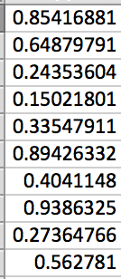
Figure 3.56:

In an adjacent column, we first find the mean $\bar{x}$ .

Figure 3.57:

Notice that the formula has $(x_{i}-\bar{x})^{2}$ for each data value $x_{i}$ . Using auto-fill in Excel, we create a column that computes this part of the expression for each data value. Notice that we call the mean $\bar{x}$ in each expression.

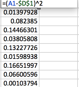
Figure 3.58:

Adding up this column and dividing by $9$ will result in the sample variance for the randomly generated data. (Note that $n=10$ and $n-1=9$ .)

Figure 3.59:
(b)

A random sample of 100 using $\tt{\color{red}\colorlet{pgfstrokecolor}{.}RAND()}$ in Excel.

We use the command $\tt{\color{red}\colorlet{pgfstrokecolor}{.}VAR.S(\ldots)}$ and leave it to the reader to verify the command is true. ¹³¹³Note that there is also a $\tt{\color{red}\colorlet{pgfstrokecolor}{.}VAR.P(\ldots)}$ . This is for the case when your sample is actually the entire population.. Part of the generated random sample of 100 and the associated sample variance of all 100 data values is then shown in Figure 3.60.

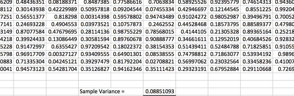
Figure 3.60:

Comparing (a) and (b), we notice that the sample variance is around 0.08. The random samples you obtain should also be somewhat close to 0.08 in sample variance.

$\clubsuit$

Mathematically, variance is a great tool for describing how spread out the data in a sample is. However, in day-to-day talk, the variance has one flaw that is commonly missed. It is not in the same units of measurement as the original data! For example, if the original sample taken was in feet, then the sample variance would actually be in feet squared. This is due to the squaring in the expression in the definition for sample variance. A better way of expressing how far apart the data is in the same units of measurement as the data is when the sample standard deviation.

Definition (Standard Deviation).

Given a sample of $n$ data values, $x_{1},x_{2},\ldots,x_{n}$ , the sample standard deviation of the data is

s=\sqrt{\dfrac{(x_{1}-\bar{x})^{2}+(x_{2}-\bar{x})^{2}+\ldots(x_{n}-\bar{x})^{% 2}}{n-1}}=\sqrt{\dfrac{1}{n-1}\sum\limits_{i=1}^{n}(x_{i}-\bar{x})^{2}},

where $\bar{x}$ is the mean of the data.

If the data encompasses the entire population, we call it population variance, denoted as $\sigma$ , and we replace $n-1$ in the formula above with just $n$ .

Really, sample standard deviation is just the square root of sample variance. The calculation can be quickly done.

Example 3.5.2.

Let’s compute the sample standard deviation of 10 randomly generated data values using $\tt{\color{red}\colorlet{pgfstrokecolor}{.}RAND()}$ in Excel by using the formula and by using the command $\tt{\color{red}\colorlet{pgfstrokecolor}{.}STDEV.S(\ldots)}$ .

Begin by generating the random sample of 10. For simplicity, suppose it is the same as that in Figure 3.56. We saw that the sample variance was 0.085070668. Taking the square root of this number, we obtain the sample standard deviation, as desired.

Figure 3.61:

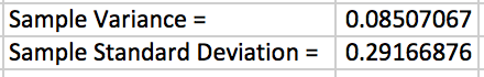
For a quicker computation, the command $\tt{\color{red}\colorlet{pgfstrokecolor}{.}STDEV.S(\ldots)}$ will also calculate the sample standard deviation. Be sure to select the original data when using the command. You should also obtain the same and as stated in Figure 3.61. $\clubsuit$

The larger the variance or standard deviation is, the more spread out the data is. Extreme outliers, therefore, will cause the variance and standard deviation to become larger even though most of the data may be concentrated in an region of the number line.

3.5.2 Quartiles

At what value is 25% of the data explained? Given a random sample, is it possible to determine a value for which 25% of the data in the sample is at or below this value? This is what quartiles will do for us.

Definition (Quartiles).

Dividing a random sample up into quarters, the values for which 25%, 50% and 75% of the data is at or below are known as quartiles and are respectively denoted as $Q1$ , $Q2$ , and $Q3$ .

We have actually messed with a quartile before but didn’t label it as such. The median is actually a quartile. It is $Q2$ . This is because when calculating the median, we are looking to see what value for which 50% of the data is at or below it.

There are many different approaches to finding $Q1$ and $Q3$ . One approach is to find the median of the lower 50% of the data and the median of the upper 50%, excluding the median of the entire sample. This will then be $Q1$ and $Q3$ , respectively. Excel calculates the $Q1$ and $Q3$ a bit differently – a method beyond the scope of this class. We will rely on calculating the quartiles without using the commands in Excel.

Example 3.5.3.

Let’s generate a random sample of 20 data with $\tt{\color{red}\colorlet{pgfstrokecolor}{.}RAND()}$ and calculate $Q1$ , $Q2$ , and $Q3$ .

In Excel, we generate a random sample of 20 data. To find $Q1$ , $Q2$ , and $Q3$ we first want to organize the data from lowest to highest in value, as seen in Figure 3.62

Figure 3.62: Sample of 20 Data

$Q2$ is the median. This can easily be calculated with the command $\tt{\color{red}\colorlet{pgfstrokecolor}{.}MEDIAN(\cdots)}$ . The authors’ obtain $Q2=0.416114567$ .

Since there are 20 data values, then the median of the entire sample is between the tenth and eleventh data value, if ordered from lowest to highest. Therefore, the lower 50% of the sample will be the first ten data values. Using $\tt{\color{red}\colorlet{pgfstrokecolor}{.}MEDIAN(\ldots)}$ again, but only on these ten values, we can obtain $Q1$ . The authors’ obtain $Q1=0.18474058$ . Following a similar approach for the upper 50%, we have $Q3=0.551750463$ . To summarize:

Q1=0.18474058

Q2=0.416114567

Q3=0.551750463

$\clubsuit$

Interquartile Range

Definition (Interquartile Range).

We define

\text{interquartile range (IQR)}=Q3-Q1.

The interquartile range describes how wide the middle 50% of the data is. Commonly, interquartile range is used to determine the presence of outliers. The following guideline is used to determine if a data value is an outlier. Let $x$ be a data value from a random sample.

x<Q1-1.5\cdot IQR

, then

x

is an outlier

x>Q3+1.5\cdot IQR

, then

x

is an outlier

Remark: The table above is used as a guideline. If a data value is ruled as an outlier, it need not be removed from the data set. More information and analysis is needed to move forward and delete data from a sample.

Example 3.5.4.

Let’s determine if the following data has any outliers.

1.3	18.3	40.3	56.7
4.2	20.1	42.4	57.8
7.7	21.0	42.9	60.8
8.7	22.8	43.7	67.3
11.5	28.3	44.7	75.3
11.5	29.9	46.2	81.3
13.5	30.5	47.2	98.2
14.5	32.5	50.7	15.0
53.3	35.4	20.2	20.5

Enter the data into Excel. We need to arrange the data from lowest to highest to determine $Q1$ and $Q3$ . Doing so, we found that $Q1=16.7$ and $Q3=49.0$ . Therefore, we have that

\text{IQR}=Q3-Q1=49.0-16.7=32.3.

It follows that

Q1-1.5\cdot IQR=-31.72775

and

Q3+1.5\cdot IQR=97.3719394.

In Excel, it is easy to see if we have any data that exceeds these values since we already have the data sorted. As a result, you should notice that 98.2 exceeds the guidelines. We would then consider this data value an outlier. However, due to how close it is to the other data along with the importance (not known here) of the data value, we may not delete it from our sample of data. $\clubsuit$

Concepts Check: 1. Find the sample standard deviation and sample variance of the data

23.1

23.2

23.3

23.4

23.5

. Answer:

s=0.158113883

s^{2}=0.025

2. Find the quartiles of the data 753.2, 55, 58, 62, 73. Answer:

Q1=54.1

Q2=58

Q3=67.5

3. Determine if the data in #2 above has any potential outliers. Answer: The value 753.2 can be deemed an outlier.

3.5.3 Exercises

1.
Answer each of the following statements as True or False.
1. (a)
  
  There is no difference in formula between population variance and sample variance.
2. (b)
  
  Sample standard deviation and sample variance are only a square root operation away from one another.
3. (c)
  
  The variance of data can be described in the same units of measurement that the data is in.
4. (d)
  
  $Q2$ has no relation to the median whatsoever.
5. (e)
  
  If a data value $x$ is deemed an outlier, then $x$ should always be removed from the data set.
2.
Without using the commands $\tt{\color{red}\colorlet{pgfstrokecolor}{.}STDEV.S}$ and $\tt{\color{red}\colorlet{pgfstrokecolor}{.}VAR.S}$ , create a spreadsheet that will compute the sample standard deviation and sample variance of a sample of 7 data values. Use it to quickly compute the sample standard deviation and sample variance of the following data.
1. (a)
  
  24.4, 15.5, 87.4, 73.4, 22.2, 81.0, 86.4
2. (b)
  
  2, 1, 3, 3, 3, 4, 3
3. (c)
  
  22.0, 21.1, 12.7, 12.0, 23.2, 15.9, 16.0
4. (d)
  
  1.0, 0.3, 0.6, 1.4, 0.4, 0.9, 1.3
3.

Using the command $\tt{\color{red}\colorlet{pgfstrokecolor}{.}=NORMINV(RAND(),20,4)}$ , generate a random sample of 900 data values. Compute the sample standard deviation, $s$ , and sample variance, $s^{2}$ . How do your values compare knowing that $\sigma=4$ and $\sigma^{2}=16$ ?
4.

Using the command $\tt{\color{red}\colorlet{pgfstrokecolor}{.}=NORMINV(RAND(),50,2)}$ , generate a random sample of 900 data values. Predict what the population standard deviation and population variance ought to be.
5.
For the following data, calculate $Q1$ , $Q2$ , and $Q3$ .
1. (a)
  
  14, 52, 66, 87, 99, 11, 1, 2, 3, 4, 5, 6, 7, 8, 26, 32, 32, 14, 88
2. (b)
  
  6, 18, 3, 6, 2, 5, 6, 8, 21, 3, 5, 10, 26, 19, 6, 13, 63, 19, 41, 91
3. (c)
  
  1,2, 2, 2, 3, 3, 4, 5, 5, 6, 8, 12, 19, 19, 21, 22, 35, 50, 61, 83
6.

Using the data in the previous example, determine if there are any outliers based on the guidelines stated in this section.