14 Regression 14.2 Finding Regression Line 14.4 (Optional) Linear Regression in Excel Alternatives

14.3 Correlation

Goals:

\bullet

Learn what correlation is;

\bullet

Learn how to analyze correlation subjectively and objectively;

\bullet

Learn how to calculate the linear correlation coefficient using Excel and Python;

Along with identifying a regression line, it is important to wonder how good of a fit a line is with the data. This is where correlation comes in.

Definition.

Correlation An objective measurement that determines how much change in the dependent variable is attributed to changes in the independent variable.

When we measure for correlation, particularly linear correlation, there are several scenarios we may encounter.

•

Positive Linear Correlation

Two variables are positively correlated when, as the $X$ variable increases in value, so does the $Y$ variable. Some examples of a positive correlation would be study time and grades; hours worked at an hourly paying job and the amount of money you get paid, etc. A positive correlation would look like this:

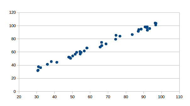
Figure 14.11: Positive Linear correlation
•

Negative Linear Correlation

Two variables are negatively correlated when, as the $X$ variable increases in value, the $Y$ variable decreases in value. Some negatively correlated variables would be: The number of people helping you move and ther time it takes to finish the move; medicine dosage and time to relief; more time practicing swimming and swim race times; etc. A negative correlation would look like this:

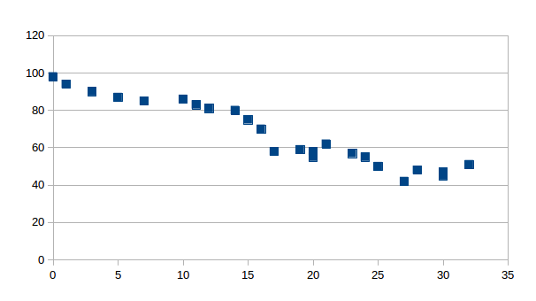
Figure 14.12: Negative Linear correlation
•

No Linear Correlation

Some variables appear to be neither positively nor negatively correlated. Sometimes there is no pattern at all, and other times there is an apparent pattern but it is not linear. ⁵⁶⁵⁶See Figure 14.2 for an example of no linear correlation. Even if we have an apparent random nonlinear pattern in our scatterplot, we cannot say that there is no correlation between the two variables. We need to say that there is no linear correlation between the two variables. Even a graph like Figure 14.13 might have a valid function that accurately describes its behavior.

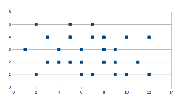
Figure 14.13: No Linear Correlation

Each of these scenarios are presented with a scatterplot. From observing the scatterplot, one can make a subjective interpretation as to which type of correlation they are encountering. But, each of these scatterplots can be open to interpretation. Where one person sees a pattern, another may not. We need a method that is objective, or impervious to personal bias. It turns out that there is such an approach. We can compute the correlation coefficient of two (or more) variables.

Definition.

Correlation Coefficient for Linear Regression The linear relationship between two variables is measured by the correlation coefficient

r=\frac{\sum{xy}-\frac{1}{n}\sum{x}\sum{y}}{\sqrt{\sum{x^{2}}-\frac{1}{n}(\sum% {x})^{2}}\sqrt{\sum{y^{2}}-\frac{1}{n}(\sum{y})^{2}}}.

(14.4)

Notice that the numerator for $r$ is the same as the numerator for $r$ in Eq. 14.2. This means that, since the denominator of each is never negative, $r$ and $b$ always have the same sign. This is an important detail to remember. This makes sense since $b$ is the slope of the regression line and $r$ describes the relationship between the two variables as positive, negative or something else.

Example 14.3.1.

Let’s use Excel to compute $r$ for the data in Example 14.2.1.

Solution. Recall that we derived the regression line for the data as

\hat{Y}=3.0+1.7X.

Notice that $b=1.7$ , which is positive. So $r$ should be positive as well. Let’s compute $r$ to check. There is no need to recalculate sums as we did in Example 14.2.1. Figure 14.6 already states all the necessary values. Using these and plugging them appropriately into Eq. 14.4 for $r$ , we have

$r=\frac{\sum{xy}-\frac{1}{n}\sum{x}\sum{y}}{\sqrt{\sum{x^{2}}-\frac{1}{n}(\sum% {x})^{2}}\sqrt{\sum{y^{2}}-\frac{1}{n}(\sum{y})^{2}}}=\frac{\sum{464}-\frac{1}% {5}{(30)}{(66)}}{\sqrt{{220}-\frac{1}{5}(30)^{2}}\sqrt{{990}-\frac{1}{5}(66)^{% 2}}}=\frac{68}{68.93475}=0.98644$

This can be done easily by cell-referencing the values from the spreadsheet created in Example 14.2.1. Pay attention to how parentheses are used. $\clubsuit$

So what does $r$ tells us exactly? The correlation coefficient, $r$ , is a measure of how spread out the data points are from the best fit line. Larger values of $|r|$ will have dots closer to the regression line; smaller values of $|r|$ will be dispersed farther from the regression line. If $r$ is around 0, then we say there is no linear correlation between the two variables. There may be a relationship between the two variables (sine, logarithmic, etc.), but it is not a linear relationship. It may turn out that there is no correlation at all between the variables, but we are unable to determine that definitely with this simple test. Finally, if $|r|$ is closer to $1$ , then there is strong evidence that the relationship between $X$ and $Y$ is linear. We state below a summarization of these ideas along with a rough classification of different $r$ values.

•

$-1\leq r\leq 1$
•

$|r|\geq 0.70\Rightarrow$ strong linear correlation
•

$|r|\approx 0.50\Rightarrow$ moderate linear correlation
•

$|r|\leq 0.25\Rightarrow$ weak linear correlation

We note that the classification of $r$ values stated above is open to interpretation based on the data. For example, if we were verifying a physical law that exhibits a linear relationship between variables, then obtaining an $r$ -value that is around $0.7$ is not a very strong value. We would be expecting a higher value.

Caution When Interpreting Correlation

It is important to remember that even if two variables are strongly correlated, there may not be a causal relationship between them. For example, you may notice that it always seems to rain when you wear a red shirt or plan a company picnic, etc. Those things (shirt color and event plan) obviously have no effect on the weather or whether it will rain or not. This is an easy mistake to make, particularly when you really want to show a causal relationship or you are convinced that one exists. One needs to be very careful with this. In fact, we state

Correlation Does Not Imply Causation

to remind ourselves of this.

In addition, establishing a correlation between two variables is the first necessary step in showing that changes in $X$ cause changes in $Y$ . It can be thought of as having veto power: If no correlation can be shown (not necessarily a linear one), then there is no point in continuing the effort to show causation.

14.3.1 Exercises

1.
Answer the following as True or False.
1. (a)
  
  $r$ can be greater than 2.
2. (b)
  
  If $r=0$ , it is still possible for two variables to be correlated, just not linearly.
3. (c)
  
  If $r=1$ , then two variables are negatively, linearly correlated.
4. (d)
  
  If two variables are in no way related to one another, such as t-shirt color and weather that day, then $r$ will always be zero.
5. (e)
  
  Scatterplots don’t offer any correlation evidence.
2.

Calculate the correlation coefficients for 2(a), (b), and (c) in the previous section. Interpret each of your results.
3.

Create a Python script that imports $X$ data and $Y$ data and calculates the correlation coefficient between the data. Have the correlation coefficient be printed out in a nice format. Test it on several data sets you have already computed the correlation coefficient for in Excel.