14 Regression 14.1 Curve of Best Fit 14.3 Correlation

14.2 Finding Regression Line

Goals:

\bullet

Learn the equation of a line;

\bullet

Learn how to how to identify the slope and intercept and what they mean;

\bullet

Learn how to find the formula for the regression line in Excel and Python.

Linear regression, or sometimes referred to as the least-squares regression line⁵³⁵³See optional section at the end of the chapter on the derivation of the linear regression formula for clarification as to why it is called the least-squares regression line. aims at finding a linear relationship between the random variables $X$ and $Y$ . That is, we are looking for $b$ and $a$ so that we can write the expression⁵⁴⁵⁴This is the equation of a line. In the previous section, we wrote it as $Y=mX+b$ , the usual way it is written in an algebra course. Due to other uses in statistics of the letters $m$ and $b$ , we avoid writing it in this manner.

\hat{Y}=bX+a.

(14.1)

In order to do just that, we need to assume we have data $x_{1},x_{2},\ldots,x_{n}$ from a random variable $X$ and $y_{1},y_{2},\ldots,y_{n}$ from a random variable $Y$ such that $x_{i}$ is paired with $y_{i}$ , for $i=1,\ldots n$ . Writing these as pairs, we have

(x_{1},y_{1}),(x_{2},y_{2}),\ldots,(x_{n},y_{n}).

From this data, we can easily calculate the values of $b$ and $a$ in Eq. (14.1).

Definition (Formula for $b$ ).

The slope, or the value $b$ , in Eq. (14.1) is calculated using the formula

b=\dfrac{n\sum xy-\sum x\sum y}{n\sum x^{2}-(\sum x)^{2}},

(14.2)

where $n$ is the number of data values, and

		$\displaystyle\sum x=x_{1}+x_{2}+\cdots+x_{n},$
		$\displaystyle\sum y=y_{1}+y_{2}+\cdots+y_{n},$
		$\displaystyle\sum xy=x_{1}y_{1}+x_{2}y_{2}+\cdots x_{n}y_{n},$
		$\displaystyle\sum x^{2}=x_{1}^{2}+x_{2}^{2}+\cdots x_{n}^{2}.$

Caution!!! Be aware that there is a difference between $\sum x^{2}$ and $(\sum x)^{2}$ .

Definition (Formula for $a$ ).

The $Y$ -intercept, or the value of $a$ , in Eq. (14.1) is calculated using the formula

a=\bar{y}-b\bar{x},

(14.3)

where $\bar{x}=\frac{1}{n}\sum x$ , $\bar{y}=\frac{1}{n}\sum y$ , and $b$ is the value obtained from the formula for the slope.

The derivation of these formulas comes from finding the least-squared distance between each of the points, $(x_{i},y_{i})$ and a line of best fit. The line that minimizes the distance from each of the points is the line that gives us the values for $a$ and $b$ above.⁵⁵⁵⁵For a more thorough derivation and reasoning behind where these formulas come from, please see the optional section on the derivation of the linear regression line at the end of the chapter. Please note that this section requires a knowledge of calculus.

Having computed the values for $a$ and $b$ in our predictive equation, we now have the equation of the line that best fits our data points. The purpose of doing this is so that we can make predictions about the value of $\hat{Y}$ given the value of $X$ . We need to be careful, though. The predictions we make are only valid for the range of data values sampled from the variable $X$ to derive the regression line equation. We can make predictions for values of $X$ outside this range, but these predictions may not be valid because we don’t know the behavior of the system outside the range of $X$ values that we originally collected. The system may flatten out, or become vertical, or exhibit sinusoidal behavior. We simply don’t know; therefore predictions using values of outside our original range should carefully analyzed.

Let’s practice using the formulas with an example.

Example 14.2.1.

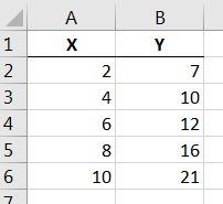
In Excel, create a scatterplot and find the equation of the regression line given the following data.

$X$	2	4	6	8	10
$Y$	7	10	12	16	21

Solution. Before we calculate the linear regression equation, it is ideal to first analyze the data by creating a scatterplot to see if the data looks somewhat linear. As we will learn later, there are statistical measurement tools we can use to determine how good a fit the regression line is to the data.

Begin by entering the data in the table above in columns $\tt{\color{red}\colorlet{pgfstrokecolor}{.}A}$ and $\tt{\color{red}\colorlet{pgfstrokecolor}{.}B}$ as shown in Figure 14.4 below.

Highlight just the data in the table and select first option within the scatterplot button located under the Insert tab on the ribbon. After doing so and adding a titles we arrive at the scatterplot of the data as seen in Figure 14.5 below.

Figure 14.5: Scatterplot of our example data

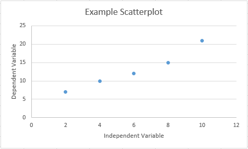
It can be seen that the points fall nearly on a straight line, but not quite. It seems appropriate that a line would fit the data. Note that the equation that we derive from these data will give somewhat accurate predictions for $y$ given $x$ , but it will not be perfect.

In order to calculate the expression for $b$ , it is useful calculate what $X^{2}$ , $Y^{2}$ , and $X Y$ are for each of the data values. Hence, we can expand our table in Excel to include these values, including the sums of each of the columns.

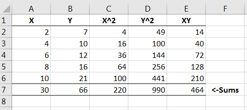
Figure 14.6: Expanded Data for Calculating $b$

Note that in our formula for $b$ , $\sum x=30$ , as seen in cell $\tt{\color{red}\colorlet{pgfstrokecolor}{.}A7}$ in Figure 14.6. A similar deduction can be made for the rest of the values in the formula for $b$ . Plugging in the necessary sums from Figure 14.6 into the formula for $b$ and noting that $n=5$ , we have

$b=\dfrac{n\sum{xy}-\sum{x}\sum{y}}{n\sum{x^{2}}-(\sum{x})^{2}}=\dfrac{5(464)-(% 30)(66)}{5(220)-(30)^{2}}=\dfrac{68}{40}=1.7.$

So the slope of our regression line is 1.7. Using this, we have that

a=\bar{y}-b\bar{x}=\dfrac{1}{n}\sum{y}-b\left(\dfrac{1}{n}\sum{x}\right)=\frac% {1}{5}(66)-(1.7)\left(\dfrac{1}{5}(30)\right)=13.2-(1.7)(6)=3.0.

Now we have the equation of our regression line:

\hat{Y}=3.0+1.7X

$\clubsuit$

Once we have the regression line, we can use it to make predictions. From the previous example, we could use the equation to make predictions for $Y$ given $X$ by plugging in values for $X$ .

		$\displaystyle\hat{y}(5)=3+1.7*5=11.5$
		$\displaystyle\hat{y}(9)=3+1.7*9=18.3.$

We need to remember, though, that only values that fall within our range of data for $X$ are valid to use. Extrapolations beyond our original range of values may not accurately reflect the relationship between $X$ and $Y$ . This is because we don’t know if, perhaps, the random variables $X$ and $Y$ exhibit a nonlinear behavior outside of our range of data.

We can also use Python to find the regression line.

Example 14.2.2.

Write a script in Python to find the line of best fit for the same data as in Figure 14.4.

Solution. Open a text editing software, such as notepad in Windows and enter in the data from Figure 14.4, as shown below, as columns with one space between each of the values, row-wise. (We used notepad.)

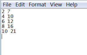
Save the file as data1.txt to a directory that you can find on your computer.

Open a script in Python and save it as Regression.py. Make sure you save it in the same directory your data file is saved. At the prompt, enter the following.

		from scipy.stats import *
		from numpy import *

These commands will load the scipy.stats and numpy modules. To import the data from the data1.txt file in Python as variables, enter the following.

x,y = loadtxt("data1.txt", unpack=True)

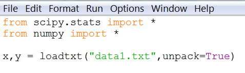
This command, when ran, loads the data from the data1.txt file into two variables: $x$ and $y$ , column-wise.

The regression function in Python returns the slope of the regression line and the intercept. In addition, it also returns the correlation coefficient and two other values that we are not interested in at the moment. Since the command requires that we account for all five of these values when we run the function on the lists $x$ and $y$ , we assign appropriate variables to each. For now, we will only focus on the slope and the intercept, $b$ and $a$ .

b,a,r,p,s = linregress(x,y)

Let’s have the slope and intercept printed out. Type the following.

print "The slope of the line is %f and the intercept is %f." %(b,a)

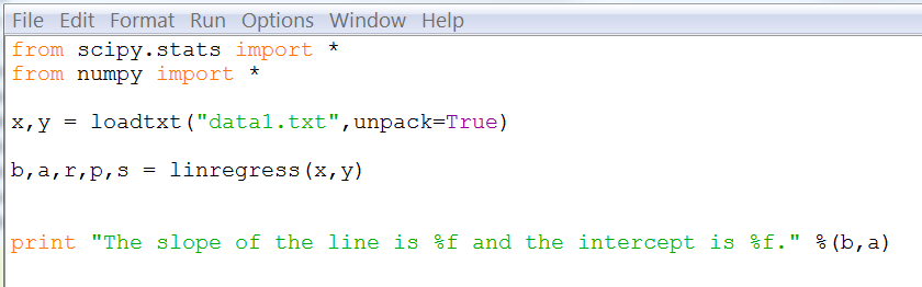
Run the script and you should obtain the same results that we have in the previous example.

Figure 14.10: Python Results

$\clubsuit$

14.2.1 Exercises

1.
Answer the following as True or False.
1. (a)
  
  Regression curves can be used for prediction purposes.
2. (b)
  
  The $a$ in Eq. 14.1 is the $X$ -intercept.
3. (c)
  
  The slope of a line, $b$ , in Eq. 14.1 can never be negative.
4. (d)
  
  There is no difference between $\left(\sum x\right)^{2}$ and $\sum x^{2}$ .
5. (e)
  
  When creating the regression line, $n$ pertains to the number of data values obtained from random variable $X$ .

Create a regression line in Excel for each of the following data sets using the tactics discussed in Example 14.2.1. Be sure to write your answer in $\hat{Y}=bX+a$ form when finished.

(a)

$X$	22.3	19.4	18.1	21.5	24.3	25.0	19.6
$Y$	82.1	100.4	109.2	90.3	74.9	66.5	108.3

(b)

$X$ 12.3 13.2 14.1 17.9 15.7 18.8 19.2

$Y$ 6.7 7.3 8.4 10.6 9.5 12.8 14.1
(c)

$X$ 26 23 24 22 21 20 19 17 14 12

$Y$ 36 37 32 39 34 41 42 46 49 52

3.

In Excel, the commands $\tt{\color{red}\colorlet{pgfstrokecolor}{.}SLOPE}$ and $\tt{\color{red}\colorlet{pgfstrokecolor}{.}INTERCEPT}$ calculate Eqs. (14.2) and (14.3), respectively. Repeat the last exercise using these shortcut commands. You should obtain the same values you have obtained in the previous exercise. Note that this is an easy way to check your answer.
4.

Explain what occurs when attempting to compute the regression line for the following data. Why would this be?

$X$ 1 1 1 1 1 1

$Y$ 3 4 5 6 7 8
5.

Instead of using the linregress command in Python, write a Python script file that loads a data file and calculates the regression line manually by using Eqs. (14.2) and (14.3). Note this involves adding up data values likened to Figure 14.6. Use the data in Example 14.2.1 for debugging purposes.

$X$	12.3	13.2	14.1	17.9	15.7	18.8	19.2
$Y$	6.7	7.3	8.4	10.6	9.5	12.8	14.1