14.4 (Optional) Linear Regression in Excel Alternatives
| Goal: |
|
There are several ways to perform linear regression in Excel. In this section, we will state many of the ways regression lines can be calculated in Excel.5757We make no attempt at showing all of the possible ways of calculating regression lines. These are just a sample of the possibilities. So far, we have seen two ways of doing regression lines.
-
•
Perform all of the calculations manually. That is, breaking formulas down into their respective parts and having Excel calculate it. This has been demonstrated in the previous sections, see Example 14.2.1 for more detail.
-
•
Use shortcut commands such as , , and . These are left as exercises, see exercises for Section 1.2 and 1.3.
Here are some additional methods we could use. We will address them one at a time using the following data.
| 2 | 4 | 6 | 8 | 10 | |
| 7 | 10 | 12 | 15 | 21 |
Scatterplot Method
This approach is relatively fast and useful. The downside of using this approach is that the numbers given for the regression equation typically suffer a little from round-off error. Here is how we do this method.
-
•
First, we need to make a scatterplot of the data. Once we have our scatterplot, we simply right click on one of the data points and then select Add Trendline in the dialog box that pops up.
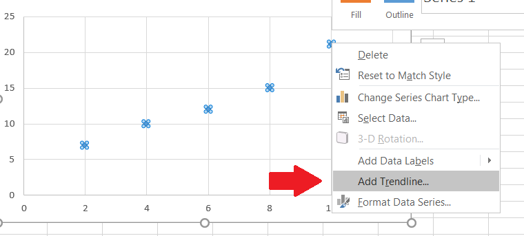
Figure 14.14: Right-click Menu Add Trendline -
•
Next, the default setting with the Trendline function is linear, but we can apply it to other types of graphs as well. Make sure linear is selected. Also, check off the boxes at the bottom of the dialog box that are labeled Display Equation on chart and Display value on chart.
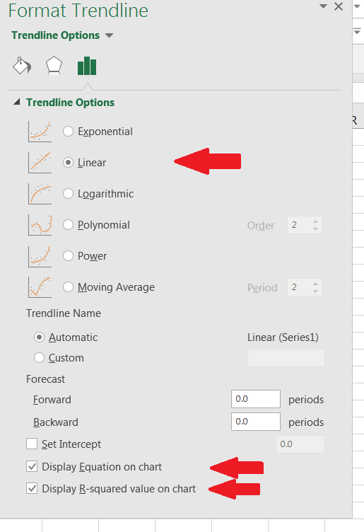
Figure 14.15: Select Options The -value is the square of the correlation coefficient. Note that still shows if the data is weak-to-strong linear correlation. However, the positive/negative relationship is lost in this data value. We can quickly get this, though, from looking at the scatterplot.
-
•
When finished, our graph looks likes this.
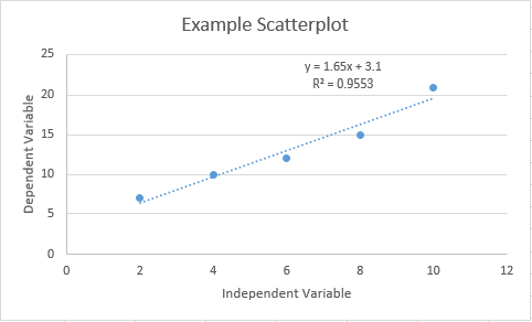
Figure 14.16: Scatterplot of our example data with trendline, regression equation, and displayed
Data Analysis Toolpak Method
This is the most thorough, useful approach of all the ones listed above. It’s also the easiest. Here is how to perform this method.
-
•
Make sure your data is entered into Excel as in Figure 14.17.
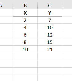
Figure 14.17: Data in Excel -
•
In the Excel Ribbon, go to Data Data Analysis Regression.
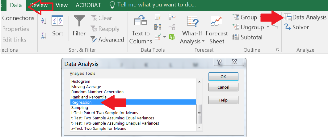
Figure 14.18: DataData Analysis -
•
Select the range of cells where the data values for are. Then select the range of cells where the data values for are. You can also select options such as residuals and residual plots. We will not be discussing these here. When finished, select OK.
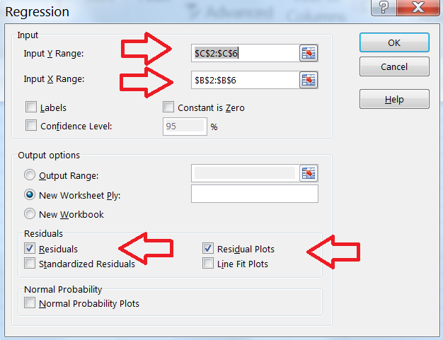
Figure 14.19: Input Data in Regression Menu -
•
Excel outputs a summary of the data on a new sheet.
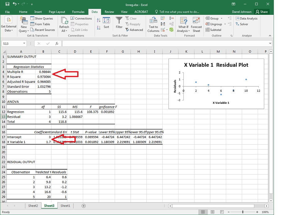
Figure 14.20: REGRESSION function output page with desired quantities highlighted The term Intercept listed in cell B17 is our a value. The term X Variable 1 in cell B18 is the slope of our line. r is given in cell B4 by the term Multiple R, and is given in cell B5 by R Square.
There are other quantities reported here that are also useful, such as the residuals, residuals plot, and others. Again, we will not be discussing them further here.
SOLVER Function
Another useful function in Excel is the Solver function. The Solver function uses numerical methods to solve equations. We can use Solver to perform regression for just about any situation (linear, sine, power law, etc.), but we will stick to linear regression here.
The process with Solver is to make a reasonable guess for and , use those guesses to make predictions for , compute the errors, and have Solver minimize those errors by adjusting our guesses for and . We need to square the errors (actual values - our predicted values) so that we don’t get any cancellations between positive and negative error values. Here is how we do this.
-
•
First, set up your worksheet as in Figure 14.21.
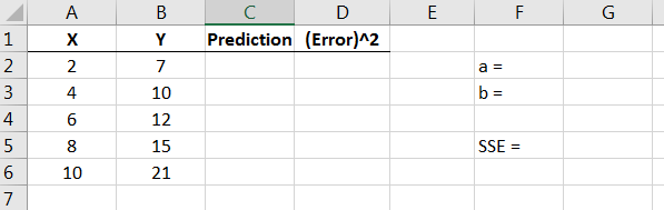
Figure 14.21: SOLVER function setup page -
•
Now we make our guesses for and . Let’s choose and . Enter these values, respectively, into cells and .5858Note that this follow through is based on setting up the worksheet exactly as shown.
-
•
Next we use our guesses for and to make predictions for based on our values of .
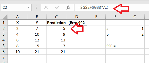
Figure 14.22: SOLVER function setup page We put dollar signs around the cell locations for and in our formula in the formula bar so that they are referred to in each cell (held constant) when we copy the formula down the column. Otherwise, Excel will move the cell references down the column and we will get a value of zero for and after a while.
-
•
Now we compute the errors between the actual values and our predicted values, then square the differences.
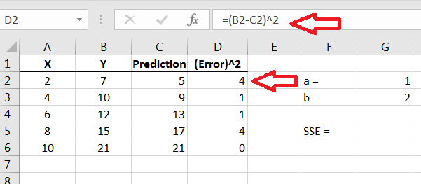
Figure 14.23: Computing the errors between and our predicted values -
•
Now we can sum up the squared errors. This is the sum of the squared errors, or SSE for short.
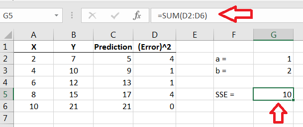
Figure 14.24: Sum of the squared errors -
•
We can now use the SOLVER function to compute and . We access the Solver function by going to Data Solver, then filling out the boxes correctly. Make sure that you are on the SSE cell when you start.
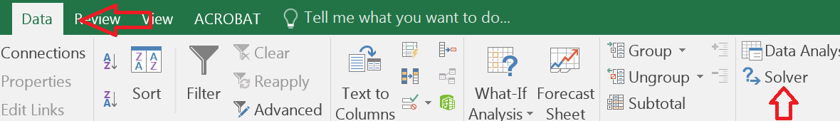
Figure 14.25: Solver Function The Objective is the cell where you computed SSE; you need to set Solver to Min by changing the values in the cells where and are. Make sure to uncheck the box that says Make Unconstrained Variables Non-Negative.
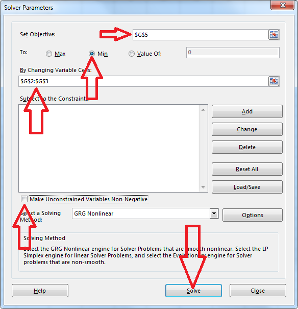
Figure 14.26: Solver function setup page -
•
Finally, we end up withe the correct values for and .
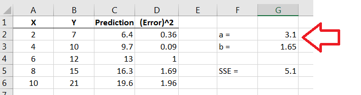
Figure 14.27: Solver results with the correct values for and
SOLVER can be used for any type of regression. It can be confusing at first, but once mastered, it is really quite straightforward.