10.5 T-Test on a Single Population Mean

A company has committed to purchase an industrial glue if there is strong evidence to support that the mean sealing strength, at a room temperature of 100 ${}^{\circ }$F, is greater than 20 lb/${\text{in}}^2.$ Following are the sealing strengths, measured in lb/${\text{in}}^2,$ of a sample of 15 tested at 100 ${}^{\circ }$F:

At a level of 5%, test whether the company should purchase the glue.

Solution: With a sample of size 15, a $T$-test is appropriate if we can assume that the population of all glue strengths is approximately normally distributed. Unless the sample size is too small, a low-road, yet reasonable approach is to create a frequency histogram of the sample, and qualitatively assess whether it looks like the sample came from a normally distributed population. Figure 10.24 gives such a graph for the sample, using a small number of bins since the sample is small.

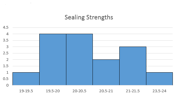
And, indeed, it doesn’t appear unreasonable to assume the sample came from a normally distributed population, i.e., we will use a $T$-test.⁴⁵⁴⁵Section 10.9 will provide another qualitative approach on whether the normality assumption is reasonable.

If $\mu$ denotes the mean for the population of sealing strengths of the glue, then the hypotheses are as follows:

Note that the direction of extreme is to the right. From the sample we have $n=15,$ $\overline{x}\approx 20.57,$ and $s\approx \mathrm{1.15.}$ Thus, the test statistic is

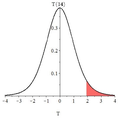
The $p$-value is the chance of observing $t_0(14)=1.90,$ or anything larger, assuming $H_0$ is true, i.e., the $p$-value is $T(14)$

The $p$-value is shown if Figure 10.25.

Using the Excel command $𝚃.\mathrm{𝙳𝙸𝚂𝚃}$ we can compute the corresponding $p$-value, as shown in Figure 10.26.

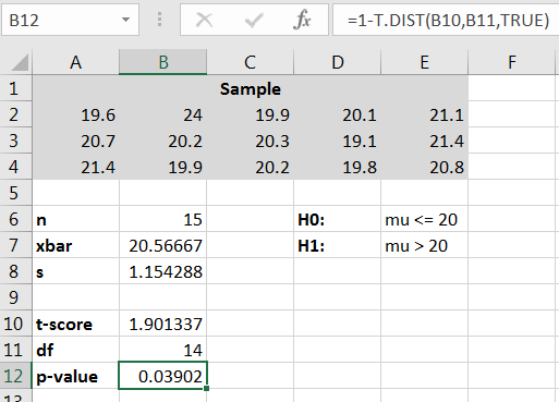
The $p$-value $\approx 0.0390,$ and since $\alpha =0.05,$ we reject $H_0.$ There is significant evidence ($t(14)=1.90,$ $p=0.0390$) that the true mean glue strength, at a room temperature of 100 ${}^{\circ }$F, is greater than 20 lb/${\text{in}}^2.$ $\mathrm{♣}$

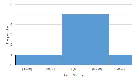
Mathematical skills assessment tests were given to a sample first grade children at the end of the school year. Their scores were as follows.

At the 10% level of significance, is there a significant evidence that in the true mean of scores on the mathematical skills assessment exam is less than 60?

Solution: With a sample of size 13, a $T$-test is appropriate if we can assume that the population of all exam scores is approximately normally distributed. Figure 10.27 gives frequency histogram for the sample, it does appear reasonable to assume the sample came from a normally distributed population.

If $\mu$ denotes the mean for the population of exam scores, then the hypotheses are as follows:

Note that the direction of extreme is to the left. From the sample we have $n=13,$ $\overline{x}\approx 57.1,$ and $s\approx \mathrm{8.5.}$ Thus, the test statistic is

The $p$-value is the chance of observing $t_0(12)=-1.25,$ or anything smaller, assuming $H_0$ is true, i.e., the $p$-value is

The $p$-value is shown if Figure 10.28.

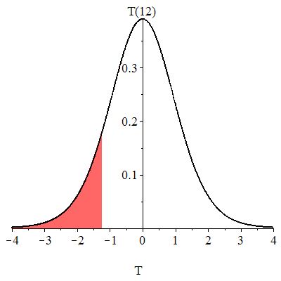
Figure 10.29 illustrates the computation of the $p$-value in Excel.

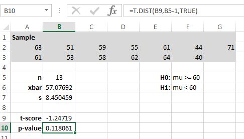
The $p$-value $\approx 0.1181$ and $\alpha =0.10,$ so we fail to reject $H_0.$ There is insufficient evidence ($t(12)=-1.25,$ $p=0.1181$) that the mean exam score is less than 60. $\mathrm{♣}$

Using the data from Example 10.5.2 on page 10.5.2, but instead use a two-sided direction of extreme, i.e., suppose the hypotheses are:

Compute the corresponding $p$-value.

Solution: The calculation of the test statistic is the same, i.e.,

The $p$-value is the chance of observing $-1.25$ or smaller, together with the chance of observing 1.25 or larger, assuming $H_0$ is true. The $p$-value is illustrated in Figure 10.30.

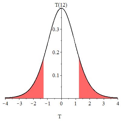
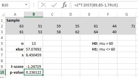
Figure 10.31 shows a method for computing the $p$-value using Excel. Note that the command computes the area of one tale (the area to the left of $-1.25$), then using the symmetry of the $t$-distribution, the result is multiplied by 2.

$\mathrm{♣}$