10 Testing a Single Population Mean 10.3 Hypotheses Setups 10.5 T-Test on a Single Population Mean

10.4 Z-Test on a Single Population Mean

This section will develop the Z-Test on a Single Population Mean (or simply $Z$ -Test), which was partially illustrated in Section 10.2. This test is appropriate if and only if one can reasonably assume that the population of sample means are normally distributed (or approximately normally distributed).

Suppose that $X$ represents a large population of numbers with unknown mean $\mu$ and standard deviation $\sigma.$ Suppose that we are going to take a simple random sample of size $n$ from $X,$ and then use that sample to do a $Z$ -Test on $\mu.$ When can we assume that the population of sample means $\bar{X}$ will be normally distributed, or approximately normally distributed?

•

If $X$ is normally distributed, then the population of sample means $\bar{X}$ will be exactly normally distributed with mean $\mu_{\bar{X}}=\mu$ and standard deviation $\sigma_{\bar{X}}=\sigma/\sqrt{n}.$
•

If $X$ is not normally distributed, but the sample size is sufficiently large, then by the Central Limit Theorem, the population of sample means $\bar{X}$ will be approximately normally distributed with mean $\mu_{\bar{X}}=\mu$ and standard deviation $\sigma_{\bar{X}}=\sigma/\sqrt{n}.$ The rule-of-thumb for “sufficiently large” we’ll us is $n\geq 30,$ but 30 might not be large enough if the population is too pathological.

In symbols, if either assumptions are met, then $\bar{X}\sim N(\mu,\sigma/\sqrt{n}).$

Bottom-line on using a $Z$ -Test: In order use a $Z$ -Test, $\sigma$ must be known, and the population must be normal or the sample size sufficiently large. If $\sigma$ is unknown, do not use a $Z$ -Test.

10.4.1 The Test Statistic and $p$ -value

If we can assume that

\bar{X}\sim N\left(\mu,\frac{\sigma}{\sqrt{n}}\right),

then the random variable

Z=\frac{\bar{X}-\mu}{\sigma/\sqrt{n}}

(10.2)

will have a standard normal distribution, i.e., $Z\sim N(0,1).$ The random variable $Z$ is used for the test statistic in a $Z$ -Test.

Recall that the $p$ -value is the chance of observing the test statistic, or anything more extreme, assuming $H_{0}$ is true. The $p$ -value depends on these three parts: (1) the value of the test statistic, (2) the direction of extreme, and (3) $H_{0}.$

We’ll examine the $p$ -value computation in each of the three different setups for $H_{0}.$

Case: Direction of Extreme to the Left

\begin{array}[]{l}H_{0}:\mu\geq\mu_{0}\\ H_{1}:\mu<\mu_{0}\\ \end{array}

If $H_{0}$ is true, then $\mu\geq\mu_{0}.$ Remember that the population mean $\mu$ is a fixed value. If $\mu\geq\mu_{0},$ then the larger $\mu$ is, the stronger the evidence the observed sample mean, $\bar{x},$ is against $H_{0},$ that is, the weakest evidence $\bar{x}$ provides against $H_{0}$ occurs when $\mu=\mu_{0}.$ Since we don’t want to reject $H_{0}$ unless there is strong evidence to do so, we assume $\mu=\mu_{0}$ in computing the $p$ -value. This maximizes the value of the computed $p$ -value, thus holding the observed evidence to the strongest standard in deciding whether to reject $H_{0}.$

Bottom line: In computing the $p$ -value, in assuming $H_{0}$ is true, we assume the $\mu=\mu_{0}.$

To compute the $p$ -value then, we use $\mu=\mu_{0}$ in Equation (10.2):

Z=\frac{\bar{X}-\mu_{0}}{\sigma/\sqrt{n}}

The observed value of $\bar{x}$ is used to compute the corresponding observed test statistic, $z_{0},$ as given below:

z_{0}=\frac{\bar{x}-\mu_{0}}{\sigma/\sqrt{n}}

(10.3)

Using $\bar{x}$ to Compute a $p$ -value

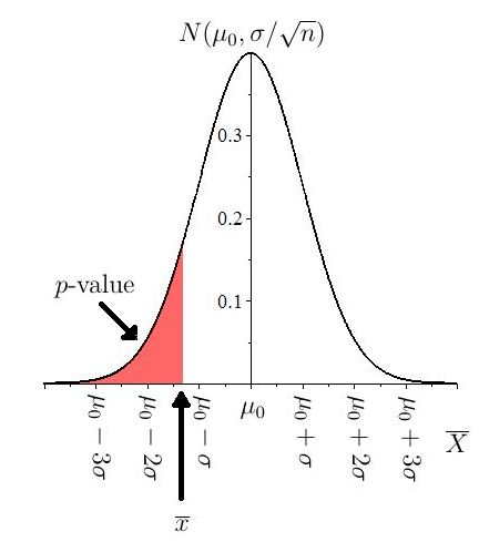
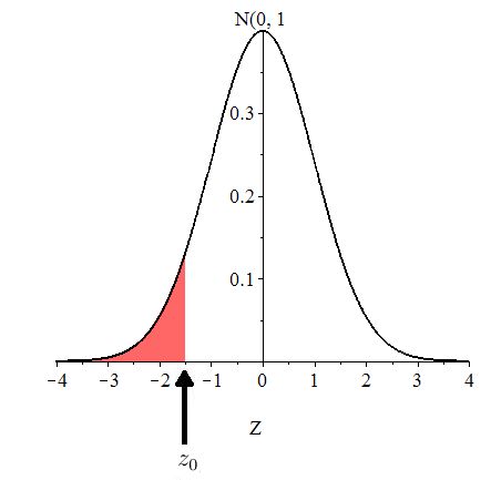
There are two ways we can compute the $p$ -value. The first method uses the observed sample mean $\bar{x}.$ In this case, the $p$ -value is the chance of observing $\bar{x},$ or anything more extreme(smaller), assuming $H_{0}$ is true ( $\mu=\mu_{0}$ ). If $\bar{X}\sim N(\mu_{0},\sigma/\sqrt{n}),$ then the $p$ -value is

P(\bar{X}\leq\bar{x})=\mbox{area under }N(\mu_{0},\sigma/\sqrt{n})\mbox{ to % the left of }\bar{x}

This is shown graphically in Figure 10.5.

Figure 10.5: $p$ -value using the distribution of $\bar{X}$

Example 10.4.1.

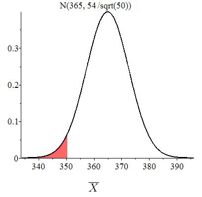
A company advertises that their product will last at least 1 year before breaking, but a consumer protection agency suspects fraud. To test this, the agency took a random sample of size 50 of the product, and the average number of days until failure was 350.4 with a sample standard deviation of 54.1. At the significance level of 5%, test whether the company is guilty of fraud. For mysterious reasons, it is known that the population standard deviation is $\sigma=54.0.$

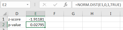
Solution: Recall from Example 10.3.1 on page 10.3.1 that $H_{0}$ is the claim that $\mu\geq 365.$ Since the sample size of $50$ is at least 30, the distribution for the sample means $\bar{X}$ is approximately $N(365,54.0/\sqrt{50}).$ Now the observed sample mean is $\bar{x}=350.4,$ so the $p$ -value is

P(\bar{X}\leq 350.4)=\mbox{area under }N(365,54.0/\sqrt{50})\mbox{ to the left% of }350.4.

The $p$ -value is shown in Figure 10.6.

Recall that we can use Microsoft’s Excel to compute areas under normal distributions using the command $\tt{\color{red}\colorlet{pgfstrokecolor}{.}NORM.DIST}$ , as shown in Figure 10.7.

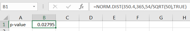
Thus, the $p$ -value is approximately 0.0280. Since $\alpha=0.05,$ we would reject $H_{0},$ and conclude that there is significant evidence that the company is guilty of fraud. $\clubsuit$

Using $z_{0}$ to Compute a $p$ -value

Note that in the calculations above, it wasn’t necessary to compute the test statistic $z_{0}$ to find the $p$ -value. But, in modern scholarly work, it is still commonly expected that the value of the test statistic be reported together with the found $p$ -value. The test statistic in Equation (10.3) can be used to compute the corresponding $p$ -value, which we will demonstrate now.

The $z$ -score for the observed sample mean $\bar{x}=350.4$ is

z_{0}=\frac{\bar{x}-\mu_{0}}{\sigma/\sqrt{n}}=\frac{350.4-365}{54/\sqrt{50}}% \approx-1.91,

as shown in Figure 10.8.

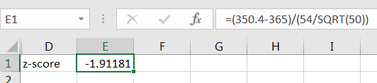
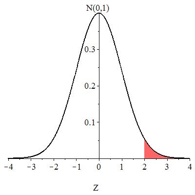
The $p$ -value is the chance of observing $z_{0}=-1.91,$ or anything more extreme (smaller), assuming $H_{0}$ is true ( $\mu=365).$ That is, the $p$ -value is

P(Z\leq-1.91)=\mbox{area under }N(0,1)\mbox{ to the left of }-1.91,

as shown in Figure 10.9.

The calculation in Excel is given in Figure 10.10.

So, the same $p$ -value is gotten, and $H_{0}$ is rejected. Here’s how the result might be presented in a scientific journal: There is significant evidence ( $Z=-1.91,$ $p=0.0280$ ) that the average time for the product to break is less than 1 year.

Concepts Check: 1. Suppose that in a

Z

-Test, the

p

-value is found to be 0.0558. If

\alpha=5\%,

what is the conclusion of the test? Answer: Fail to reject

H_{0}.

2. Suppose that in a

Z

-Test, the value of

z_{0}

obtained is

-1.78.

If the direction of extreme is to the left, as a probability, describe the corresponding

p

-value. Answer: The

p

-value is the probability of observing

-1.78,

or anything smaller, assuming

H_{0}

is true. 3. Suppose that in a

Z

-Test, the value of

z_{0}

obtained is

-1.78.

If the direction of extreme is to the left, as an area under a curve, describe the corresponding

p

-value? Answer: The

p

-value is the area under

N(0,1)

to the left of

-1.78.

4. Suppose that in a

Z

-Test, the value of

z_{0}

obtained is

-1.78.

If the direction of extreme is to the left, what Excel command will compute the corresponding

p

-value? Answer:

\tt{\color{red}\colorlet{pgfstrokecolor}{.}=NORM.DIST(-1.78,0,1,TRUE)}

5. Suppose the in a

Z

-Test,

H_{0}

is the claim that

\mu\leq 40.0,

and the summary statistics for the sample are

\bar{x}=45.3,

s=6.6,

and

n=35.

What is the value of the test statistic? Answer:

\displaystyle{z_{0}=\frac{45.3-40.0}{6.6/\sqrt{35}}\approx 4.75}

Case: Direction of Extreme to the Right

\begin{array}[]{l}H_{0}:\mu\leq\mu_{0}\\ H_{1}:\mu>\mu_{0}\\ \end{array}

If the direction of extreme is to the right, the calculations are handled identically as given previously, except that $p$ -values are areas to the right. The subtlety here is that the Excel command $\tt{\color{red}\colorlet{pgfstrokecolor}{.}NORM.DIST}$ gives area to the left, which we must remember so that a correct $p$ -value is computed.

Example 10.4.2.

A pet food manufacturer claims that each can of cat food they make contains 6 ounces of product. The manufacturer is concerned that the cans are being overfilled, so the company randomly selects 25 cans and measures the contents. The sample average and sample standard deviation for the sample are 6.20 and 0.51 ounces, respectively. At a level of 5%. test whether there is significant evidence that the cans are, on average, being overfilled. It is reasonable to assume that the population of ounces of food in cans is normal, and for reasons unknown, the population standard deviation is known to be $\sigma=0.50.$

Solution: From Example 10.3.2 on page 10.3.2, the null hypotheses $H_{0}$ is $\mu\leq 6$ and the direction of extreme to the right. Since the population is normal and $\sigma$ is known, we can use a $Z$ -Test. Since we need to compute a $z$ -score anyhow, we will consistently use the $z$ -score to compute the $p$ -value.

The $z$ -score for the observed sample mean $\bar{x}=6.20$ is

z_{0}=\frac{6.2-6}{0.5/\sqrt{25}}=2.0.

The $p$ -value is the chance of observing $z_{0}=2.0,$ or anything more extreme (larger), assuming $H_{0}$ is true ( $\mu=6).$ That is, the $p$ -value is

P(Z\geq 2.0)=\mbox{area under }N(0,1)\mbox{ to the right of }2.0,

as shown in Figure 10.9.

The calculation in Excel is given in Figure 10.12.

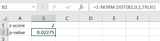
Since the $p$ -value is $\leq\alpha,$ we reject $H_{0}.$ That is, there is significant evidence ( $Z=2.0,$ $p=0.0228$ ) that the true average amount of food in the cans is greater than 6 ounces.

$\clubsuit$

Case: Two-Sided Direction of Extreme

\begin{array}[]{l}H_{0}:\mu=\mu_{0}\\ H_{1}:\mu\neq\mu_{0}\\ \end{array}

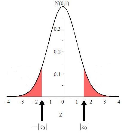
If the direction of extreme is two-sided, then $H_{0}$ is of the form $\mu=\mu_{0}.$ In this case, sample means $\bar{x}$ that are larger or smaller than $\mu_{0}$ give evidence against $H_{0}.$ Equivalently values of $z_{0}$ larger or smaller than 0 provide evidence against $H_{0}.$ So to compute a corresponding $p$ -value, we compute area of the tail more extreme than $z_{0},$ and the area of the tail more extreme than the symmetric value of $z_{0},$ $-z_{0}.$ More precisely, under the curve $N(0,1),$ the $p$ -value is the combined area to the right of $|z_{0}|$ and to the left of $-|z_{0}|.$ Figure 10.13 illustrates.

Example 10.4.3.

Let’s use the sample summary data from Example 10.4.2 on page 10.4.2, but use a two-sided direction of extreme. That is, suppose the competing hypotheses are:

\begin{array}[]{ll}H_{0}:&\mu=6\\ H_{1}:&\mu\neq 6\\ \end{array}

For purposes of illustration, let’s perform the hypothesis test using $\alpha=0.01.$

Solution: The calculation of the test statistic is unchanged, i.e., the test statistic is still

z_{0}=\frac{6.20-6}{0.50/\sqrt{25}}=2.0.

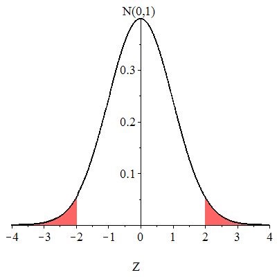
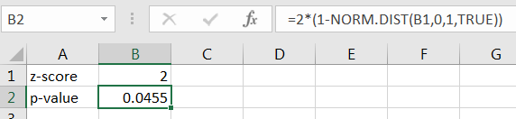
Since the direction of extreme is two-sided, however, the $p$ -value is the chance of observing $2.0$ or anything larger, together with the chance of observing $-2.0$ or anything smaller, assuming $H_{0}$ is true. The $p$ -value is illustrated in Figure 10.14.

The calculation in Figure 10.15 computes the area to the right of $2.0,$ then using the symmetry of the standard normal distribution $N(0,1),$ multiplies the result by 2.

Figure 10.15: Two-tailed calculation in Excel

Since the $p$ -value is greater than $\alpha,$ we fail to reject $H_{0}.$ Thus, there is insufficient evidence ( $Z=2.0,$ $p=0.0455$ ) that the true mean amount of food in the cans is different than 6 ounces. $\clubsuit$

Bottom line for when a

Z

-test on a single population mean is appropriate: • The population

X

is known to be normally distributed, or the sample size is sufficiently large (

\geq 30

). • The population standard deviation

\sigma

is known.

Exercises

1.
A psychologist is studying the distribution of IQ scores of girls at an alternative school. They want to test the hypothesis that the average IQ score is higher than 105. A random sample of 34 girls is taken and their sample average score was 106 with a sample standard deviation of 14. It is known that the population standard deviation is 15.
1. (a)
  
  What is the population of interest?
2. (b)
  
  State the competing hypotheses.
3. (c)
  
  What is the direction of extreme?
4. (d)
  
  Why is it reasonable to use a $Z$ -Test?
5. (e)
  
  Compute the test statistic and corresponding $p$ -value.
6. (f)
  
  Sketch the $p$ -value.
7. (g)
  
  State your conclusion at the $\alpha=0.05$ level.
8. (h)
  
  State the conclusion in a manner appropriate for a scientific journal.
9. (i)
  
  What type of error could have been made?
2.
Colleges frequently provide estimates of student expenses such as housing. A local community college claims that the average student housing expense per month is $650. To test the claim, a consultant is hired. The consultant samples 200 students yielding a sample mean of $611.63 and sample standard deviation $132.85. It is known that the population standard deviation is $130.0.
1. (a)
  
  What is the population of interest?
2. (b)
  
  State the competing hypotheses.
3. (c)
  
  What is the direction of extreme?
4. (d)
  
  Why is it reasonable to use a $Z$ -Test?
5. (e)
  
  Compute the test statistic and corresponding $p$ -value.
6. (f)
  
  Sketch the $p$ -value.
7. (g)
  
  State your conclusion at the 5% significance level.
8. (h)
  
  State the conclusion in a manner appropriate for a scientific journal.
9. (i)
  
  What type of error could have been made?
3.
A company’s service technicians took an average of 1.8 hours to respond to trouble calls from business customers who had purchased service contracts. The CEO of the company believes that the average response time this year has decreased. A simple random sample size of 35 of independent response times from business customers is selected, yielding a sample mean and sample standard deviation of of 1.5 hours and 0.5 hours, respectively. It is known that the population standard deviation is 0.52 hours.
1. (a)
  
  What is the population of interest?
2. (b)
  
  State the competing hypotheses.
3. (c)
  
  What is the direction of extreme?
4. (d)
  
  Why is it reasonable to use a $Z$ -Test?
5. (e)
  
  Compute the test statistic and corresponding $p$ -value.
6. (f)
  
  Sketch the $p$ -value.
7. (g)
  
  State your conclusion at the $\alpha=0.05$ level.
8. (h)
  
  State the conclusion in a manner appropriate for a scientific journal.
9. (i)
  
  What type of error could have been made?
4.
The Survey of Study Habits and Attitudes (SSHA) is a psychological test that measures the motivations, attitude toward school, and study habits of students. Scores range from 0 to 200. The mean score for U.S. college students is about 115. A teacher who suspects that older students have better attitudes toward school gives the SSHA to 25 students who are at least 30 years of age. Their sample mean score is 133.2, with sample standard deviation 32.0. It is known that the population of scores for students at least 30 years of age is normally distributed and that the population standard deviation is 35.
1. (a)
  
  What is the population of interest?
2. (b)
  
  State the competing hypotheses.
3. (c)
  
  What is the direction of extreme?
4. (d)
  
  Why is it reasonable to use a $Z$ -Test?
5. (e)
  
  Compute the test statistic and corresponding $p$ -value.
6. (f)
  
  Sketch the $p$ -value.
7. (g)
  
  State your conclusion at the $\alpha=0.10$ level.
8. (h)
  
  State the conclusion in a manner appropriate for a scientific journal.
9. (i)
  
  What type of error could have been made?
5.
The average yield of corn in the U.S. is about 135 bushels per acre (BPA). A survey of 25 farmers this year gives a sample mean yield of 138.4 BPA and sample standard deviation yield of 15.1 BPA. We want to know whether this is good evidence that the national mean this year is not 135 bushels per acre. Assume that the farmers surveyed are a simple random sample from the population of all commercial corn growers, and that the population of bushels per acre is normally distributed. It is known that the population standard deviation is 15.0 BPA.
1. (a)
  
  What is the population of interest?
2. (b)
  
  State the competing hypotheses.
3. (c)
  
  What is the direction of extreme?
4. (d)
  
  Why is it reasonable to use a $Z$ -Test?
5. (e)
  
  Compute the test statistic and corresponding $p$ -value.
6. (f)
  
  Sketch the $p$ -value.
7. (g)
  
  State your conclusion at the 10% level.
8. (h)
  
  State the conclusion in a manner appropriate for a scientific journal.
9. (i)
  
  What type of error could have been made?

10.4.2 Decision Rules and Critical Values

Recall that a decision rule is a description of the values for either $\bar{X}$ or $Z$ for which a null hypothesis $H_{0}$ will be rejected. The collection of these values is called a rejection region. A value of $\bar{x}^{*}$ or $z^{*}$ that delineates between rejecting and failing to reject $H_{0}$ is called a critical value.

These terms don’t add anything new structurally to hypothesis testing, but they are terms used by some scientists. Hence, we should be familiar with their meanings.

Case: Direction of Extreme to the Left

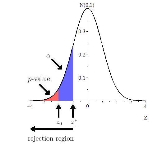
Suppose that $H_{0}$ is the claim that $\mu\geq\mu_{0}.$ Note that the direction of extreme is to the left. Suppose that the significance level $\alpha$ is given. In order to reject $H_{0},$ we would need that the observed $p$ -value is $\leq\alpha,$ so the largest possible $p$ -value that still results in rejecting $H_{0}$ is if the $p$ -value is equal to $\alpha.$ Let $z^{*}$ denote the value of $Z$ that gives a $p$ -value equal to $\alpha,$ i.e.,

\alpha=P(Z\leq z^{*})=\mbox{ area to the left of }z^{*}\mbox{ under }N(0,1).

This is shown in Figure 10.16.

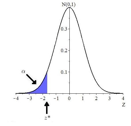
For an observed $z_{0},$ $H_{0}$ is rejected if and only $z_{0}\leq z^{*},$ because the $p$ -value is $\leq\alpha$ if and only if $z_{0}\leq z^{*}.$ This interval, $(-\infty,z^{*}),$ is called the rejection region. Figure 10.17 illustrates.

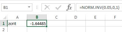
Figure 10.17: Red area $+$ blue area = $\alpha.$

We can use the Excel command $\tt{\color{red}\colorlet{pgfstrokecolor}{.}NORM.INV}$ to compute $z^{*}.$ For example, if $\alpha=0.05,$ then $z^{*}\approx-1.6449$ as shown in Figure 10.18.

If $z^{*}$ is known, then Equation (10.3) can used to compute the critical value, $\bar{x}^{*},$ for $\bar{X}:$

z^{*}=\frac{\bar{x}^{*}-\mu_{0}}{\sigma/\sqrt{n}}

(10.4)

The critical value $\bar{x}^{*}$ works similarly, i.e., $H_{0}$ is rejected if and only if the observed sample mean $\bar{x}$ is less than or equal to $\bar{x}^{*}.$

Example 10.4.4.

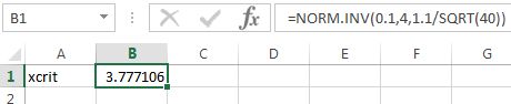
Suppose that $H_{0}:\mu\geq 4$ and $\alpha=0.10.$ Suppose a random sample of size $40$ yields a sample mean of 3.9, and suppose it is known that $\sigma=1.1.$ Use $x^{*}$ to decide on whether to reject $H_{0}.$

Solution: Using Excel, we have $z^{*}=\tt{\color{red}\colorlet{pgfstrokecolor}{.}NORM.INV(0.1,0,1)}\approx-1.28.$ Equation (10.4) gives

-1.28=\frac{\bar{x}^{*}-4}{1.1/\sqrt{40}}

and hence, $x^{*}\approx 3.78.$ Since the direction of extreme is to the left, the rejection region is all real numbers less than or equal to 3.78. The observed sample mean of 3.9 falls outside of the rejection region, so we fail to reject $H_{0}.$ $\clubsuit$

Remark: In Example 10.4.4, $x^{*}$ can be found directly using $\tt{\color{red}\colorlet{pgfstrokecolor}{.}NORM.INV}$ , as shown in Figure 10.19. Note that computation uses the assumption that the $H_{0}$ is true in similar fashion to computing a $p$ -value, i.e., $\mu_{0}=4$ is used for the population mean $\mu,$ and $\sigma/\sqrt{n}=1.1/\sqrt{40}$ for the standard deviation.

Figure 10.19:

x^{*}

using

\tt{\color{red}\colorlet{pgfstrokecolor}{.}NORM.INV}

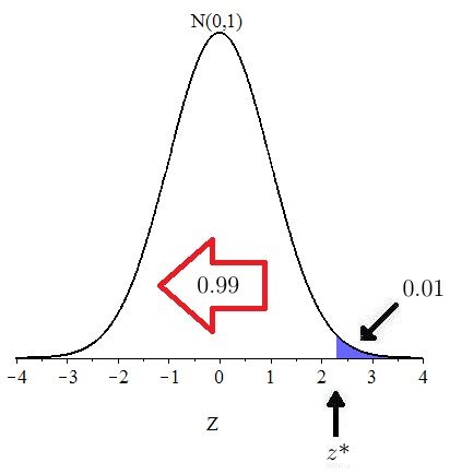
Case: Direction of Extreme to the Right

The only change here is that the direction of extreme switches the inequalities. For example, if the direction of extreme is to the right, then $z^{*}$ is chosen so that

\alpha=P(Z\geq z^{*})=\mbox{area to the right of }z^{*}\mbox{ under }N(0,1).

Figure 10.20 illustrates.

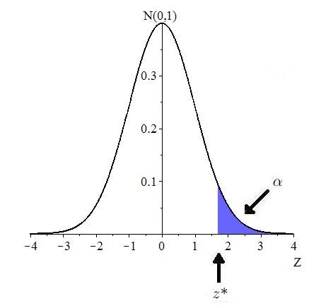
For example, suppose $\alpha=0.01$ and the direction of extreme is to the right. Then

z^{*}=\tt{\color{red}\colorlet{pgfstrokecolor}{.}NORM.INV(0.99,0,1)}\approx 2.% 3263,

as illustrated in Figure 10.21.

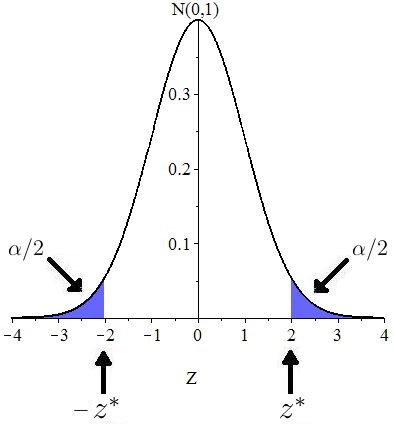
Figure 10.21: $z^{*}=\tt{\color{red}\colorlet{pgfstrokecolor}{.}NORM.INV(0.99,0,1)}$

Case: Two-sided Direction of Extreme

If the direction of extreme is two-sided, then in order to determine the value of $z^{*},$ the significance level $\alpha$ is split in half over the two tales. This is shown in Figure 10.22.

Figure 10.22: Two-sided Direction of Extreme

Example 10.4.5.

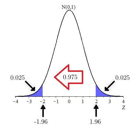
Suppose the direction of extreme is two-sided and that $\alpha=0.05.$ Compute $z^{*}.$

Solution: The area in each tail is $\alpha/2=0.025,$ so the area to the left of $z^{*}$ is $0.975,$ as shown in Figure 10.23.

Using Excel, the value of $z^{*}$ can be computed using $\tt{\color{red}\colorlet{pgfstrokecolor}{.}NORM.INV}$ as follows:

z^{*}=\tt{\color{red}\colorlet{pgfstrokecolor}{.}NORM.INV(0.975,0,1)}\approx 1% .96.

$\clubsuit$

In the Concepts Check below, assume that has been determined appropriate to use a $Z$ -Test.

Concepts Check: 1. Suppose the direction of extreme is to the left. If

\alpha=0.2,

what is the value of

z^{*}?

Answer:

z^{*}=\tt{\color{red}\colorlet{pgfstrokecolor}{.}NORM.INV(0.2,0,1)}\approx-0.8% 416

2. Suppose the direction of extreme is to the right. If

\alpha=0.15,

what is the value of

z^{*}?

Answer:

z^{*}=\tt{\color{red}\colorlet{pgfstrokecolor}{.}NORM.INV(0.85,0,1)}\approx 1.% 0364

3. Suppose the direction of extreme is two-sided. If

\alpha=0.1,

what is the value of

z^{*}?

Answer:

z^{*}=\tt{\color{red}\colorlet{pgfstrokecolor}{.}NORM.INV(0.95,0,1)}\approx 1.% 6449

4. Suppose the direction of extreme is to the left. If

\alpha=0.2,

what is the decision rule? Answer:

z^{*}=-0.8416

(from Problem 1). The decision rule is, “Reject

H_{0}

if the observed

z_{0}

is less than or equal to

-0.8416.

” 5. Suppose the direction of extreme is two-sided. If

\alpha=0.1,

what is the decision rule? Answer:

z^{*}=1.6449

(from Problem 3). The decision rule is, “Reject

H_{0}

if the observed

z_{0}

is less than or equal to

-1.6449

or greater or equal to

1.6449

.” 6. Suppose that the direction of extreme is to the left. It is determined that

z^{*}=3.1,

and from a sample of size

30,

z_{0}=3.3

is observed. What decision is made? Answer: Fail to reject

H_{0}

, because

z_{0}\not\leq z^{*}.

7. Suppose that

H_{0}

is the claim

\mu\leq 10

and that

\alpha=0.15

has been chosen. If a sample of size

n=50

is selected, yielding a sample mean of

10.4,

what is the approximate value of

\bar{x}^{*}?

Assume

\sigma=2.0

Answer: The direction of extreme is to the right, and for

\alpha=0.15

the value of

z^{*}\approx 1.0364

(from Problem 2). Using Equation 10.4, we have

1.0364=\frac{\bar{x}^{*}-10}{2.0/\sqrt{50}},

and solving for

\bar{x}^{*}

gives

\bar{x}^{*}\approx 10.29.

Or, equivalently, the Excel command

\tt{\color{red}\colorlet{pgfstrokecolor}{.}NORM.INV(0.85,10,2/SQRT(50))}

yields that same result.

Exercises

1.
A psychologist is studying the distribution of IQ scores of girls at an alternative school. They want to test the hypothesis that the average IQ score is higher than 105. A random sample of 34 girls is taken and their average score was 106 with a standard deviation of 14. Use $\alpha=0.05$ and and assume $\sigma=15.$
1. (a)
  
  What is the value of $z^{*}?$
2. (b)
  
  In terms of $z^{*},$ what is the decision rule?
3. (c)
  
  What is the rejection region?
4. (d)
  
  What is the relationship between the decision rule and the rejection region?
2.
Colleges frequently provide estimates of student expenses such as housing. A local community college claims that the average student housing expense per month is $650. To test the claim, a consultant is hired. The consultant samples 200 students yielding a sample mean of $611.63 and sample standard deviation $132.85. Use $\alpha=0.05$ and assume $\sigma=130.$
1. (a)
  
  What is the approximate value of $x^{*}?$
2. (b)
  
  In terms of $x^{*},$ what is the decision rule?
3. (c)
  
  Using part (b) and the observed sample mean, what is the decision made?
3.
A company’s service technicians took an average of 1.8 hours to respond to trouble calls from business customers who had purchased service contracts. The CEO of the company believes that the average response time this year has decreased. A simple random sample size of 35 of independent response times from business customers is selected, yielding a sample mean and sample standard deviation of of 1.5 hours and 0.5 hours, respectively. Use $\alpha=0.1$ and assume $\sigma=1.$
1. (a)
  
  What is the value of $z^{*}?$
2. (b)
  
  In terms of $z^{*},$ what is the decision rule?
3. (c)
  
  Using part (b) and the observed sample mean, what is the decision made?
4.
The Survey of Study Habits and Attitudes (SSHA) is a psychological test that measures the motivations, attitude toward school, and study habits of students. Scores range from 0 to 200. The mean score for U.S. college students is about 115. A teacher who suspects that older students have better attitudes toward school gives the SSHA to 30 students who are at least 25 years of age. Their sample mean score is 133.2, with sample standard deviation 32.0. Use $\alpha=0.05$ and assume $\sigma=30.$
1. (a)
  
  What is the approximate value of $x^{*}?$
2. (b)
  
  In terms of $x^{*},$ what is the decision rule?
3. (c)
  
  Using part (b) and the observed sample mean, what is the decision made?

10.4 Z-Test on a Single Population Mean

10.4.1 The Test Statistic and p-value

Using x¯ to Compute a p-value

Example 10.4.1.

Using z0 to Compute a p-value

Example 10.4.2.

Example 10.4.3.

Exercises

10.4.2 Decision Rules and Critical Values

Example 10.4.4.

Example 10.4.5.

Exercises

10.4.1 The Test Statistic and $p$ -value

Using $\bar{x}$ to Compute a $p$ -value

Using $z_{0}$ to Compute a $p$ -value