10 Testing a Single Population Mean 10.5 T-Test on a Single Population Mean 10.7 Confidence Intervals and Two-Sided Hypothesis Tests

10.6 Optional: Effect Size

Statistics is powerful at detecting when two numbers are different, even if they are very close together. For example, we have a population $X$ of numbers with mean $\mu,$ and suppose that a hypothesis test is to be conducted on the following:

\begin{array}[]{ll}H_{0}:&\mu=\mu_{0}\\ H_{1}:&\mu\neq\mu_{0}\\ \end{array}

Suppose that $H_{0}$ is false, and that simple random sampling is conducted on the population. If the sample size is large enough, then with high reliability $H_{0}$ will be rejected, no matter how close together $\mu$ and $\mu_{0}$ might be. And, if the difference between $\mu$ and $\mu_{0}$ is small relative to the population standard deviation $\sigma,$ then that difference may not be of importance. That is, while results from a test may be significant, the distinction may by unimportant.

For example, suppose that a golfer wants to test, when using her driver, whether her average drive off the tee is different from 240 yards. She could generate a sample of drives off the tee, carefully measuring the distance of each. If $\mu$ denotes her true mean driving distance, then the sample could be used to test the hypotheses:

\begin{array}[]{ll}H_{0}:&\mu=240\\ H_{1}:&\mu\neq 240\\ \end{array}

Suppose that $H_{0}$ is false, and that $\mu=240.03,$ i.e., her true mean drive is about 1 inch longer than 240 yards. While 240.03 yards is definitely not equal 240 yards, is that an important difference? No. But, if she were to select a sample size that is sufficiently large, it is highly likely the statistical test would yield a significant result, i.e., a small $p$ -value.

How do we tell when a significant result is important? For example, when is the difference between 240.03 and 240 important? In this case, unless the golfer is freakishly consistent, the difference of 1 inch is small relative to the standard deviation $\sigma$ of the drive lengths. That is, the question on whether a significant result is important is made by considering the difference $\mu-\mu_{0}$ relative the standard deviation $\sigma$ within the population. Thus, if a result is significant, to measure the importance can done via Cohen’s d, which is the ratio

d=\frac{|\mu-\mu_{0}|}{\sigma}.

(10.7)

The smaller the ratio, the more that the significance is due to a large sample size; the larger the ratio, the more important the difference. In statistics, this is called measuring the effect size, which simply means estimating the degree to which the significant result is mostly due to a large sample (small effect), or that the difference is important (large effect).

Since

\mu

and

\sigma

are (usually) unknown, we estimate Cohen’s

d

using the following:

d\approx\frac{|\bar{x}-\mu_{0}|}{s}.

(10.8)

As it mimics the ratio in Equation 10.7, note that the ratio in Equation 10.8 is not especially sensitive to sample size. In Equation 10.8, if $\sigma$ is known, then use it instead of $s .$

A couple of simulations will help illustrate.

Example 10.6.1.

The purpose of the example is to show that statistical tests, such as the $T$ -test, can detect very small differences, and to show what Cohen’s $d$ does in this situation. Let’s use the golfer scenario above, and assume that the the true mean driving distance is $\mu=240.03$ yards, i.e., $|\mu-\mu_{0}|=0.03$ yards. To demonstrate the sensitivity of the $T$ -test further, suppose that the difference $|\mu-\mu_{0}|$ is small relative to $\sigma.$ For this purpose, let’s assume that $\sigma=1$ yard.

To detect such a small difference $|\mu-\mu_{0}|=0.03$ with a comparatively large $\sigma=1,$ we need a large sample size; $n=10,000$ ought to reliably work.

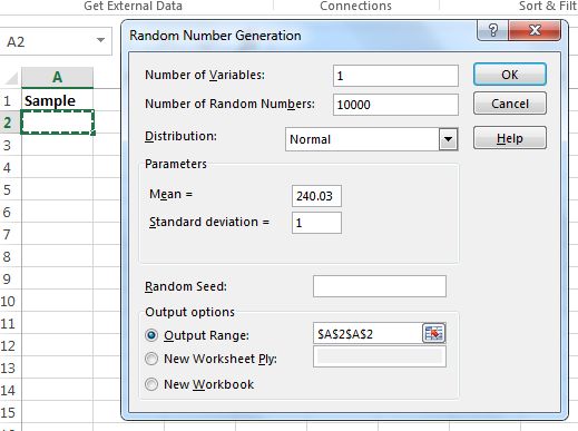
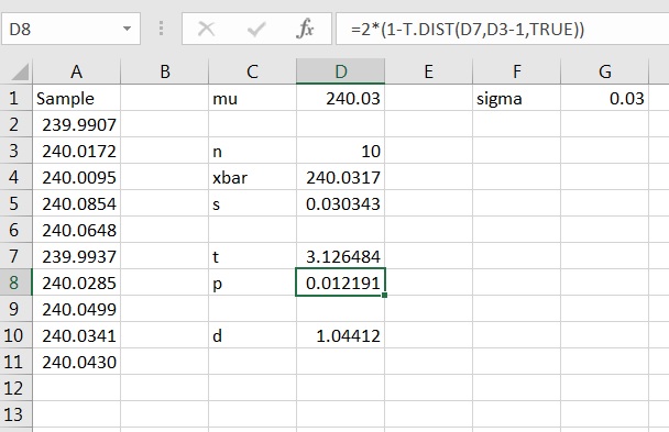
In Excel, use the Random Number Generator to generate the sample. Use $\mu=240.03$ for the mean, $\sigma=1$ for the standard deviation, and $n=10000$ for the number of random numbers, as shown in Figure 10.32.

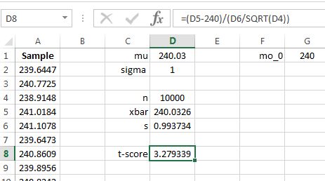
Compute the summary statistics for the sample, and then compute the test statistic, as shown in Figure 10.33.

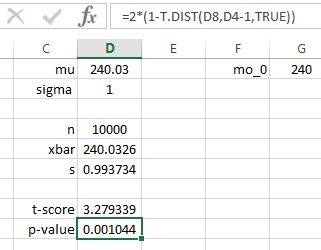
The corresponding $p$ -value is shown in Figure 10.34. You are very likely to get a small $p$ -value. If you don’t, simulating again might do the trick. Note that in the simulation displayed, the result is significant, unless a very small value of $\alpha$ was chosen.

Yet, note the approximate value of Cohen’s $d,$ ⁴⁶⁴⁶In this example, because we are in control of a simulation, the exact value of Cohen’s $d$ can be calculated. In this case, the exact value is 0.03. as shown in Figure 10.35.

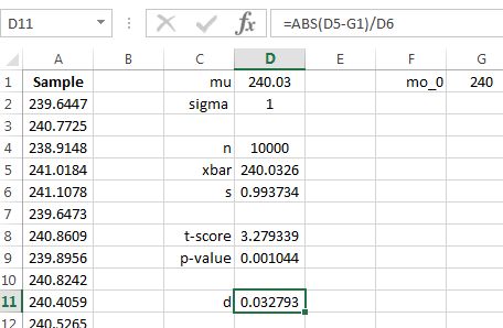
The value $d\approx 0.0327$ is small, strongly suggesting that the significant result is due mainly to a large sample size, just as expected. $\clubsuit$

Concepts Check: 1. The sample size of

n=10,000

in the simulation shown in Example 10.6.1 was chosen because of the small effect. Try some smaller sample sizes. For example, even with

n=1000,

you are likely to get a “large”

p

-value.

Example 10.6.2.

The purpose of this example is to illustrate Cohen’s $d$ when there is a large effect. We can do this using much of the setup in Example 10.6.1. Let us again set $\mu_{0}=240$ and $\mu=240.03,$ but we want the difference $|\mu-\mu_{0}|=0.03$ to be a large effect. To do that, we ought to choose $\sigma$ to be smaller, so that the difference is “large” relative to the standard deviation. To illustrate, let’s choose $\sigma=0.03.$ With this choice, the difference between $\mu$ and $\mu_{0}$ is 1 standard deviation, which we know to be a nontrivial distance in a population.

Since the effect is large, we ought to be able to detect it even with a small sample size, such as $n=10.$ Repeat the simulation in Example 10.6.1, using $n=10$ and $\sigma=0.03.$ You likely see a result as shown in Figure 10.36.

$\clubsuit$

Concepts Check: 1. Try the simulation using

\mu=10,

\mu_{0}=10.5,

and

\sigma=1.

In this case, Cohen’s

d

is going to be

d=\frac{|\mu-\mu_{0}|}{\sigma}=\frac{0.5}{1}=0.5,

that is, the effect size is moderate. Trying different sample sizes, see how large

n

needs to be in order to get a small

p

-value.

Using Cohen’s $d$

You should estimate the effect size only when you get a significant result, i.e., if you fail to reject $H_{0},$ then don’t use Cohen’s $d .$ If a result is significant, then use Formula (10.8) on page 10.8 to approximate the effect size. This is illustrated by the flowchart in Figure 10.37.

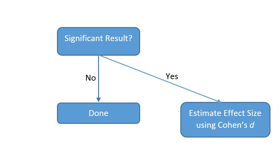
Figure 10.37: When to Estimate Effect Size

Table 10.1 gives guidelines for interpreting values of Cohen’s $d .$

$\mathbf{d}$	Effect Size
0.2	Small
0.5	Medium
0.8	Large

Table 10.1: Interpreting Cohen’s

d

Example 10.6.3.

A company has committed to purchase an industrial glue if there is strong evidence to support that the mean sealing strength, at a room temperature of 100 ${}^{\circ}$ F, is greater than 20 lb/ $\mbox{in}^{2}.$ Following are the sealing strengths, measured in lb/ $\mbox{in}^{2},$ of a sample of 10 tested at 100 ${}^{\circ}$ F:

\begin{array}[]{ccccc}21.5&21.2&19.9&21.5&18.9\\ 21.1&22.1&22.1&21.4&19.3\\ \end{array}

At a level of 5%, test whether the company should purchase the glue. If the null hypothesis is rejected, estimate the effect size.

Solution: From Example 10.5.1 on page 10.5.1, the $p$ -value is approximately 0.0166, and hence, $H_{0}$ is rejected. Thus, it is appropriate to estimate the effect size. From the calculations we have $\bar{x}=20.9$ and $s=1.13,$ and hence,

d\approx\frac{|\bar{x}-\mu_{0}|}{s}=\frac{|20.9-20|}{1.13}\approx 0.80.

This implies a large effect size, i.e., the average sealing strength surpasses the company’s minimum expectation and the company should purchase the glue. $\clubsuit$

Exercises

For each problem in the exercises from Section 10.5 on page 10.5, compute and interpret the effect size if a result the significant.