9.5 Simulations

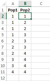
For ease of input into Excel, let’s use the populations as given in Figure 9.5 on page 9.5. Create a column for each box (population), inputting a value for each number in the box, as in Figure 9.11.

Let’s use the decision rule“reject $H_0$ if the selected number is 4 or greater,” so that $\alpha =1/10=0.1$ and $\beta =6/10=\mathrm{0.6.}$ We’ll use Excel to randomly pick a box, and then randomly select a number from the chosen box.

The primary command we will use is $\mathrm{𝙸𝙽𝙳𝙴𝚇}$. From a block of given cells, $\mathrm{𝙸𝙽𝙳𝙴𝚇}$ allows the user to select the value from a particular cell within the block. The command takes three inputs:

• •

  The first input is a block of cells from which the cell will be selected.

• •

  The second is the row from which to pick.

• •

  The third input is the column from which to pick.

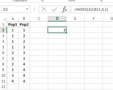
For example, $=\mathrm{𝙸𝙽𝙳𝙴𝚇}(\mathrm{𝙰𝟸}:\mathrm{𝙱𝟷𝟷},\mathrm{𝟿},\mathrm{𝟷})$ would output the value in cell $\mathrm{𝙰𝟷𝟶}$, because the ninth row in the block is row 10, and the first column is column A. The output is shown in Figure 9.12.

Now using $\mathrm{𝚁𝙰𝙽𝙳𝙱𝙴𝚃𝚆𝙴𝙴𝙽}$, we can randomly select a column and row, as shown in 9.13.

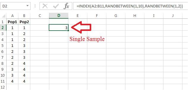
This is a simulated sample, and from it we must make a decision. Since the selected number is not 4 or greater, we would not reject $H_0,$ i.e., there is insufficient evidence to reject the hypothesis that the number came from Population 1. Note that since we failed to reject $H_0,$ a Type II error might have occurred, though since we didn’t record which box was selected, it is not possible to know if the error was made. This is the case in practice, in that when a decision is made, it is impossible to know if an error occurred. However, this is a simulation, meaning we can control what what is known, i.e., we can keep track of which population was selected, and hence, determine if an error was made.

All we need to do is remove the $\mathrm{𝚁𝙰𝙽𝙳𝙱𝙴𝚃𝚆𝙴𝙴𝙽}(\mathrm{𝟷},\mathrm{𝟸})$ from inside the $\mathrm{𝙸𝙽𝙳𝙴𝚇}$ command, so that we can see which population is chosen before the sample is generated. Figure 9.14 demonstrates.

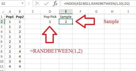
The command in cell $\mathrm{𝙳𝟸}$ selected column 1, which is then referenced in the $\mathrm{𝙴𝟸}$ command. Having chosen Population 1 makes $H_0$ true. Since a 2 was chosen from the box, we would fail to reject $H_0,$ and hence, we would make a good decision.

Note: We’re going to drag commands down, so you’ll want absolute referencing on the row numbers for the cells that refer to Population 1 and Population 2, i.e., note the $\$$’s in the $\mathrm{𝙸𝙽𝙳𝙴𝚇}$ command in Figure 9.14.

Using Excel’s $\mathrm{𝙸𝙵}$ command, we can encode the decision rule of “reject $H_0$ is a 4 or more extreme is observed.” For ease of uisng $\mathrm{𝙸𝙵}$, we’ll denote a decision as follows:

1. 1 = Fail to Reject $H_0;$

2. 2 = Reject $H_0.$

The decision rule can be executed with $\mathrm{𝙸𝙵}(\mathrm{𝙲𝙴𝙻𝙻}\ge \mathrm{𝟺},\mathrm{𝟸},\mathrm{𝟷})$, as shown in Figure 9.15.

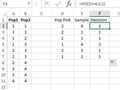
Note that the choice of encoding the decisions as above means the following: If the selected population and decision outcome are the same, then an error has not occurred. For example, if Population 1 is selected, and the decision is a 1, then an error did not occur.

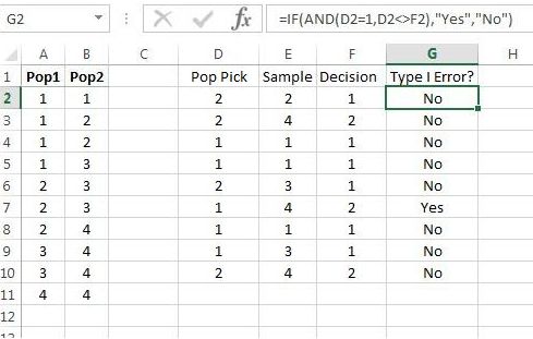
We can use $\mathrm{𝙸𝙵}$ to test whether a Type I error has occurred. Such an error has occurred if Population 1 was selected and $H_0$ was rejected. We can use Excel’s $\mathrm{𝙰𝙽𝙳}$ command to check both conditions as shown in Figure 9.16.

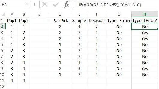
Similarly, we can check whether a Type II error has occurred, as in Figure 9.17.

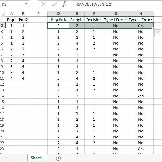
We’re now set to do a large number of simulations in Excel. Drag the commands down, as if Figure 9.18, for at least a few hundred rows.

Now use Excel to check on the following:

1. 1.

   When $H_0$ is true, a Type II error never occurs. Similarly, when $H_0$ is false, a Type I error never occurs.

2. 2.

   When $H_0$ is true, the percent of Type I errors made is about 10%, and when $H_0$ is false, the percent of Type II errors made is about 60%. (Recall that for the decision rule used in this example, $\alpha =0.1$ and $\beta =\mathrm{0.6.}$

Without too much pain, we can use the work above to simulate making decisions with samples of size 2.

First, when working with samples of size greater than 1, we will need to use summary statistics as tools. The examples used in this chapter all involve populations that consist of numbers, so computing a sample mean from sample data is a natural choice, and will be the choice in this simulation.

To make a reasonable comparison, let’s use the same setup as in Figure 9.18 on page 9.5, and the same decision rule of “reject $H_0$ if the sample mean is 4 or greater.” Only column $𝙴$ needs to modified: After the box is selected, two numbers need to be chosen from the population, and then their average computed. To make the computation much less complicated, we will allow sampling with replacement, i.e., after selecting a number from the chosen box, it is placed back into the population and can be chosen again. With this assumption, column $𝙴$ need only be changed as in Figure 9.19.

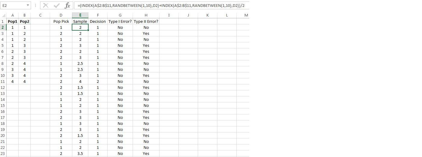
To construct the command in cell $\mathrm{𝙴𝟸}$, copy and past the $\mathrm{𝙸𝙽𝙳𝙴𝚇}$ command into the Excel formula bar, putting a plus sign between the two commands:

$$\begin{array}{c}\mathrm{𝙸𝙽𝙳𝙴𝚇}(𝙰\$\mathrm{𝟸}:𝙱\$\mathrm{𝟷𝟷},\mathrm{𝚁𝙰𝙽𝙳𝙱𝙴𝚃𝚆𝙴𝙴𝙽}(\mathrm{𝟷},\mathrm{𝟷𝟶}),\mathrm{𝙳𝟸})+\hfill \\ \mathrm{𝙸𝙽𝙳𝙴𝚇}(𝙰\$\mathrm{𝟸}:𝙱\$\mathrm{𝟷𝟷},\mathrm{𝚁𝙰𝙽𝙳𝙱𝙴𝚃𝚆𝙴𝙴𝙽}(\mathrm{𝟷},\mathrm{𝟷𝟶}),\mathrm{𝙳𝟸})\hfill \end{array}$$

Then add parentheses on the outside, and divide by 2:

$$\begin{array}{c}=(\mathrm{𝙸𝙽𝙳𝙴𝚇}(𝙰\$\mathrm{𝟸}:𝙱\$\mathrm{𝟷𝟷},\mathrm{𝚁𝙰𝙽𝙳𝙱𝙴𝚃𝚆𝙴𝙴𝙽}(\mathrm{𝟷},\mathrm{𝟷𝟶}),\mathrm{𝙳𝟸})+\hfill \\ \mathrm{𝙸𝙽𝙳𝙴𝚇}(𝙰\$\mathrm{𝟸}:𝙱\$\mathrm{𝟷𝟷},\mathrm{𝚁𝙰𝙽𝙳𝙱𝙴𝚃𝚆𝙴𝙴𝙽}(\mathrm{𝟷},\mathrm{𝟷𝟶}),\mathrm{𝙳𝟸}))/\mathrm{𝟸}\hfill \end{array}$$

Now copy the command down the rest of the column, and recompute the following:

1. 1.

   When $H_0$ is true, what is the percentage of Type I errors committed?

2. 2.

   When $H_0$ is false, what is the percentage of Type II errors committed?

You should observe percentages of errors that are greatly reduced, i.e., if the sampling process is reliable, then increasing sample size will increase confidence in making a good decision.

We can use the work done previously to quickly build a simulation for estimating $p$-values for samples of size 2. First, recall that a $p$-value is the chance of observing the test statistic, or anything more extreme, assuming $H_0$ is true. Thus, to simulate a $p$-value in this scenario, Population 1 is always chosen, and column $𝙳$ can be replaced with 1’s, as shown in 9.20.

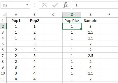
Column $𝙴$ will automatically update to simulated means for samples of size 2.

As an example computation, suppose the observed sample mean is 3.5. The corresponding $p$-value is the chance of observing 3.5 (the test statistic) or anything larger (more extreme) assuming the sample came from Population 1 ($H_0$ is assumed true). We can estimate the chance using the simulated sample means. After generating a large number of sample means, compute the proportion of means that are 3.5 or larger, which can be done using $\mathrm{𝙲𝙾𝚄𝙽𝚃𝙸𝙵}$ and $\mathrm{𝙲𝙾𝚄𝙽𝚃}$:

$=3.5")/COUNT(E:E)\}"\; display="block">=\mathrm{𝙲𝙾𝚄𝙽𝚃𝙸𝙵}(𝙴:𝙴,\mathrm{"}\ge \mathtt{3.5}\mathrm{"})/\mathrm{𝙲𝙾𝚄𝙽𝚃}(𝙴:𝙴)$

Figure 9.21 illustrates.

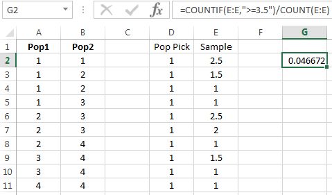
Thus, if a sample mean of 3.5 is observed from a sample of size 2, then the approximate $p$-value is 0.0467. (The estimate shown was generated from a 1307 simulated sample means.)