7 Population Models 7.5 The Normal Distribution 8 Confidence Intervals for One Parameter

7.6 The $t$ -Distribution

The normal distribution is a vital to modern statistics, but there are situations in which a different bell-shaped and symmetric distribution should be used. Suppose that population $X$ is normally distributed with mean $\mu,$ and suppose we were to take simple random samples of size $n$ from the population. Each sample would have a corresponding sample mean, and from those we can build a new random variable, $\bar{X},$ the sample means from the random samples of size $n .$ Each sample would have a sample standard deviation as well, and that too then forms a random variable, $S .$ (In this situation, the standard deviation of $X$ is unknown, and hence, cannot be used in calculations.) Using $\bar{X}$ and $S,$ a new random variable can be constructed as the ratio,

T=\dfrac{\bar{X}-\mu}{S/\sqrt{n}}.

(7.7)

This distribution was invented by William Sealy Gosset, and since he published the work under the pseudonym Student, it is commonly called the Student $t$ -distribution, but we will simply call it the $t$ -distribution. Because of the original population $X$ is normally distributed, $T$ can assume any real value, i.e., $-\infty<T<\infty.$ The $t$ -distribution depends on the sample size $n,$ though we don’t refer to the sample size directly. Instead we refer to the degrees of freedom ( $d f$ ) of the $t$ -distribution. If the sample size is $n,$ then

df=n-1.

Equation (7.7) is read as the “ $t$ -distribution with $n-1$ degrees of freedom.”

A $t$ -distribution is symmetric and bell-shaped, always with a mean of 0, regardless of the degrees of freedom. The standard deviation of a $t$ -distribution depends on the degrees of freedom. The larger $d f,$ the smaller the spread and the closer $T$ behaves like $Z,$ the standard normal distribution. Figure 8.8 depicts what happens to the $t$ -distribution as the degrees of freedom increases.

Figure 7.27: Increasing Degrees of Freedom

As with normal distributions, there are two calculations we will do with $T :$

1.

Compute an area to the left of a value under the curve, i.e., compute $P(T<t),$ where $t$ is any real number.
2.

Conversely, given an area $A,$ compute the value $t$ where $P(T<t)=A.$

The Excel commands for both are discussed next.

7.6.1 T.DIST

Working in similar fashion to NORM.DIST, Excel’s T.DIST approximates $P(T<t)$ for given values $t$ and $d f,$ with syntax as given below:

P(T<t)\approx\tt{\color{red}\colorlet{pgfstrokecolor}{.}\mbox{T.DIST}({\it t},% {\it df},\mbox{TRUE)}}

The key to remember when using this command is that it gives area to the left, just as with NORM.DIST.

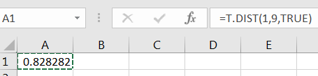
Example 7.6.1.

To compute $P(T<1)$ if $df=9,$ one would execute

P(T<t)\approx\tt{\color{red}\colorlet{pgfstrokecolor}{.}\mbox{T.DIST}(1,9,% \mbox{TRUE)}}\approx 0.828281802.

Figure 7.28: Computing $P(T<1)$ with $df=9$

$\clubsuit$

7.6.2 T.INV

As with NORM.INV, the Excel command T.INV computes a value of $t$ for a given area to the left. That is, if $A=P(T<t)$ for a given degrees of freedom $d f,$ then

t\approx\tt{\color{red}\colorlet{pgfstrokecolor}{.}\mbox{T.INV}({\it A},{\it df% })}.

Example 7.6.2.

Suppose we are working with a $t$ -distribution with $df=9.$ To compute the value of $t$ such that $P(T<t)=0.8,$ we would execute

t\approx\tt{\color{red}\colorlet{pgfstrokecolor}{.}\mbox{T.INV}(0.8,9)}\approx 0% .88340386.

In literature, you’ll see this result written as $t(9)=0.88.$

7.6.3 $t$ -distribution Simulation - Optional

The ratio given in Equation (7.7) works as advertised. We can observe this via a simulation of the ratio

t=\frac{\bar{x}-\mu}{s/\sqrt{n}},

(7.8)

where we control the population from with the samples are taken. For this to work properly, we only need that the population $X$ to be normally distributed.

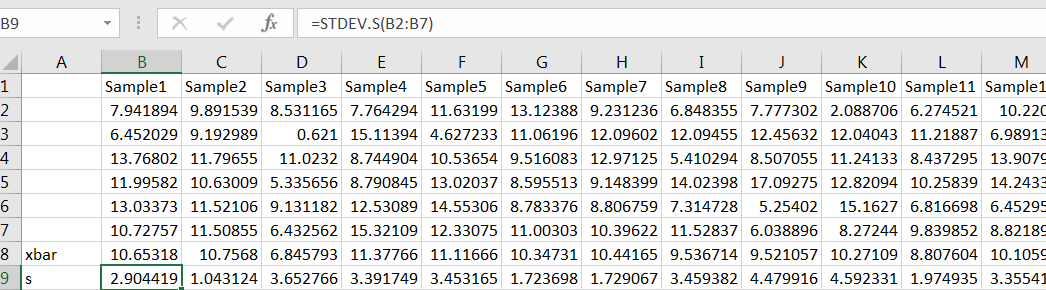
For example, let’s estimate $P(T<1)$ with $df=5$ using a simulation. For the population from which to sample, suppose that $X\sim N(10,3).$ (Pick your favorite values for $\mu$ and $\sigma,$ you need not pick 10 and 3.) For $df=5,$ we need samples of size $n=6.$ Use Excels random number generator to simulate a large number, say 1000, samples of size 6, computing $\bar{x}$ and $s$ for each sample:

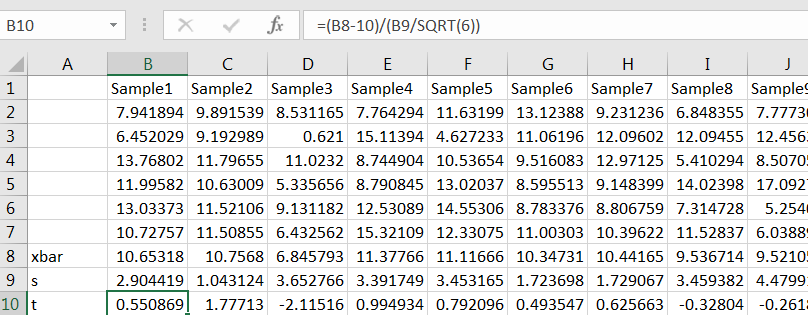
Figure 7.29: Simulation of Samples from $X\sim N(10,3)$ with $n=6$

The for each sample, compute Equation (7.8):

Now use COUNTIF to count the number of values of $t$ that are less than 1, and divide by the number of simulations to get the proportion:

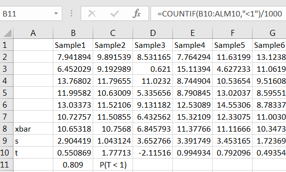
Figure 7.31: Compute the Proportion $<1$

If you used a large number of simulations, such as 1000, your estimate will likely be close to the value given by T.DIST(1,5,TRUE). Try it.