8.1 Confidence Intervals for the Mean
| Goals: |
|
When analyzing data, we would like to know what the population mean is. However, most of the time we are faced with only a sample from the population. Thus, we can only calculate a sample mean as an estimate of the actual population mean. If given a sample mean, is it possible to obtain an interval about the sample mean that attempts to show where the population mean may fall? In this section, we will study a way to do just that.
8.1.1 Is Known
Given a very large population, the sample mean, will likely never be exactly the population mean, . Our goal here is to obtain a range of values that likely represents the location of the population mean. Such a range of values is called a confidence interval.
Definition (Confidence Interval).
A range of values described by a lower value and an upper value that has a confidence in containing the population parameter. We call the confidence level of the associated confidence interval, usually written as a percentage.
Typically, we want to be small, say 0.1, 0.05, or 0.01. But there are drawbacks to being too small, as we will see.
A confidence interval for involves finding and so that
with a confidence of . But how do we go about constructing such a confidence interval? The following theorem gives us the formula used to calculate the confidence interval for the population mean, .
Theorem (Confidence Interval for , with Known).
Given a random sample , and the population standard deviation , the confidence interval for is given by
where is the sample mean and is the critical value from the standard normal distribution such that .
Remark: It is common to write the confidence interval as
where is called the margin of error of .
The most difficult part of calculating the confidence interval for , with known, is finding . The rest is basic arithmetic. We will first need to recap how to find given a confidence level of .
Finding
Recall that a -score is a random variable that is normally distributed with mean 0 and standard deviation 1. That is, . The critical value is an outcome from a -score that has the following relation to .
Definition (Critical Value: ).
We define the critical value, , as the value in which the following holds:
where is a random variable having a standard normal distribution. That is, the area under the standard normal density curve that is to the right of the critical value is .
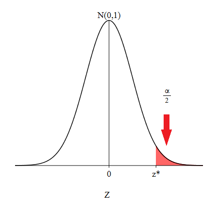
Figure 8.1 shows a representation of what stands for on a standard normal distribution. Since the standard normal distribution is symmetric about 0, there is an equal and opposite value, that stands for . If you add these two areas together, you get a combined area of . Thus, the area between and is , the confidence level we intend on having, since the total area under the standard normal density curve is 1. How does help give us a confidence interval for ? Since we have the relation
with a bit of algebra, we can manipulate the inequality within the probability statement to look like
Extracting the inequality from within the parentheses and replacing the random variable with an outcome , we have the confidence interval desired. For further explanation, see Derivation of Confidence Interval for , Known at the end of this section.
So obtaining the critical value, , is necessary in order to construct a confidence interval for . Let’s look into how to find . In Excel and Python, areas under probability density curves are calculated from the left. If we want the area under the standard normal density curve to the right of to be , then the area to the left of would be . The commands in Figure 8.2 reflect this along with reminding you of the commands used to calculate in Excel and Python.
| Compute in Excel | Compute in Python |
| norm.ppf()) |
-
•
To use the Python command, it is required that you load scipy.stats first.
Let’s practice finding in both Excel and Python.
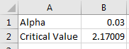
Example 8.1.1.
Given , find the associated critical value in Excel.
We first need to calculate what is. On a new sheet in Excel and in cell , type the string Alpha.
We need to first find . Since , then . In cell , type
In cell , type the string Critical Value.
In cell , use cell-referencing by typing the command
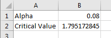
Hence, you should obtain that . Figure 8.3 represents the layout you should have in the end.
Example 8.1.2.
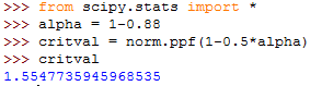
Given , find the associated critical value in Python.
Make sure you first have scipy.stats loaded. If not, type the following command.
| from scipy.stats import * |
Again, we need to find first. Based on the same relationship that , type the following in Python to compute and save to the variable alpha.
| alpha = 1-0.88 |
Compute and store the critical value, , by typing the command
| critval = norm.ppf(1-0.5*alpha) |
You should arrive at . Figure 8.4 represents the layout you should have in the end. Remember to call critval to obtain the value for .
Constructing the Confidence Interval
There are a few things that are required first in order to construct the confidence interval for , knowing :
Be sure you have the following:
-
•
Make sure your unbiased random sample is coming from a normally distributed population or the sample size is large enough ().3333It is always a good idea to assess normality first.
-
•
Make sure you have . Is it given to you?
-
•
Calculate the sample mean, , unless it is given to you.
-
•
Based on your confidence level, , calculate the critical value .
The following table recaps the commands in Excel and Python that are necessary for computing the confidence interval for the mean, with known. Each row stands for equivalent commands.
| Action | Excel Commands | Python Commands |
|---|---|---|
| Compute the Mean | mean(…) | |
| Compute the Square Root | sqrt(…) | |
| Compute | norm.ppf() |
-
•
The mean and sqrt commands require the library numpy . The norm.ppf command requires the library scipy.stats .
Let’s see a few examples of constructing confidence intervals for , known, using Excel and Python.
Example 8.1.3.
Suppose a simple random sample of 35 salaries of college football coaches, with a sample mean of , is taken from a normally distributed population. Assuming that , use Excel to find a 90% confidence interval for the mean .
It is wise to make sure that our sample comes from a normally distributed population. In this case, it is mentioned in the problem. So normality is assumed and we can proceed.
From the problem, it is understood that . Hence, . From our formula for the confidence interval, we need to find . On a new sheet in Excel, type in cell the string .
Then in cell , type the following command that will compute the critical value associated with a confidence level of .
Since the formula for the confidence interval is
let’s first compute the lower value: . In cells and , type the strings and , respectively.
With , , plug into cell the following:
Notice that we are cell-referencing the value for .
Repeat the process for the upper value in cell by typing the following:
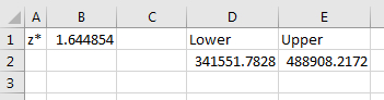
Cells and represent the lower and upper values of the confidence interval. Hence the 90% confidence interval for the population mean is . Figure 8.6 reflects the layout of the problem in Excel.
Example 8.1.4.
Colleges frequently provide estimates of student expenses such as housing. Suppose the data is normally distributed with . A simple random sample of 43 houses was collected and the sample mean for student housing was calculated to be . Construct a 87% confidence interval for , the population mean of student housing cost.
The problem states that the data are normally distributed. So we may move forward with constructing the confidence interval.
Since we are using Python, remember to load numpy and scipy.stats. If you have not yet, use the following commands to do so.
| from numpy import * | |||
| from scipy.stats import * |
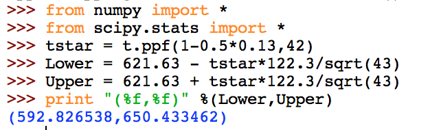
From the problem, it is understood that the . Hence . Let’s find . Type the following command that will assign the critical value, , to the variable name zstar.
| zstar = norm.ppf(1-0.5*0.13) |
Let’s name the lower value of the confidence interval as LOWER. At the prompt, type the following to assign it to LOWER.
| LOWER = 621.63 - zstar*122.3/sqrt(43) |
Repeat the process for calculating the upper value of the confidence interval. Assign it to the name UPPER.
| UPPER = 621.63 + zstar*122.3/sqrt(43) |
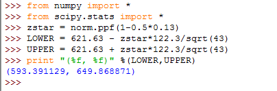
Let’s have Python print out the confidence interval. Type the following.
| print "(%f, %f)" %(LOWER,UPPER) |
You should obtain the confidence interval . Figure 8.7 represents the layout that you should have in Python.
Derivation of Confidence Interval for , Known (Optional)
You may wonder: How does this formula come to be? Recall from the Central Limit Theorem that for a sufficiently large sample size , the distribution of sample means, , becomes normal. That is,
Knowing this tells us the likelihood of obtaining different sample means. For standardization purposes, we can transform into a -score by using the following formula:
and, as a result, the random variable is normally distributed with and , or, rather
We want to be the likelihood that the -score, obtained from the sample mean calculated, lies between and , which are just -scores that correspond to and , respectively. This means that
By replacing with and manipulating the inside inequality, we have
Flipping the inside inequality around, we have
| (8.1) |
Remember that is a random variable and is an outcome from . Equation 8.1 states that out of all confidence intervals we can construct of the form
% of them will capture the population mean, . Hence, we have obtained our desired confidence interval.
8.1.2 Is Not Known
In reality, the population standard deviation, , is never known exactly. We tend to use the sample standard deviation, , as an estimate for since it’s the next best thing we can obtain. Since we are now estimating another parameter, we must adjust the way we calculation of the confidence to account for more variability. Recall that the random variable
has a -distribution with degrees of freedom. This distribution looks like standard normal distribution, . In fact as degrees of freedom, , increases, the -distribution approaches and eventually becomes the standard normal distribution. Figure 8.8 depicts what happens to the -distribution as the degrees of freedom, , increases.
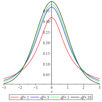
The -distribution will have fatter tails to allow for more variability due to now being an estimate for .
The process for constructing a confidence interval for will be the similar to the case when we knew . However, since we do not know we must change a couple things. The following theorem represents the changes needed in the construction of a confidence interval for , with not known.
Theorem (Confidence Interval for , with Not Known).
Given a random sample , and the associated sample standard deviation , the confidence interval for is given by
where is the sample mean and is the critical value from the Student’s -distribution with degrees of freedom such that .
Remark: Again, it is common to write the confidence interval as
where is called the margin of error of . Note that may be used interchangeably between both cases of when either is known and is not known.
Similar to constructing confidence intervals for knowing , the most difficult part of constructing confidence intervals for not knowing is finding . Let’s recap how to find given a confidence interval of and degrees of freedom .
Finding
The random variable has a -distribution with degrees of freedom . The critical value, is a particular outcome of that has the following relation to .
Definition (Critical Value: ).
We define the critical value, , as the value in which the following holds:
where is a random variable having a -distribution of degrees of freedom. That is, the area under the -distribution with degrees of freedom to the right of the critical value is .
The -distribution is also symmetric about 0, similar to that of standard normal distribution. So the symmetric value, , stands for . Hence , and thus showing the connection to the confidence level we desire out of the confidence interval.
Obtaining is definitely necessary in order to construct a confidence interval for , not knowing . In order to find , we need the degrees of freedom. Degrees of freedom is easy to calculate. Just remember,
where is the sample size taken. When calculating we will need to supply the degrees of freedom into the commands. Below the commands used to calculate in and Python.
| Compute in Excel | Compute in Python |
| t.ppf(,) |
-
•
To use the Python command, it is required that you load scipy.stats first.
Do you notice the similarity in the commands to the commands for finding ? Can you reason out why we are still using ? Also notice that second input in both commands involves telling the programs what the degrees of freedom is. In both cases, stands for the sample size.
Let’s practice finding in both Excel and Python.
Example 8.1.5.
Given , find the associated critical value in Excel knowing that the sample size taken is .
We first need to calculate what is. On a new sheet in Excel and in cell , type the string Alpha.
Since , then . In cell , type
In cell , type the string Critical Value.
Knowing that degrees of freedom is , use cell-referencing to compute by typing the following command in cell in cell :
You should obtain . Figure 8.10 represents the layout in Excel you should have in the end.
Example 8.1.6.
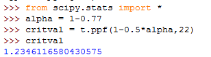
Given , find the associated critical value in Python knowing that the sample size taken is .
Make sure you first have scipy.stats loaded. If not, type the following command.
| from scipy.stats import * |
We need to find first. Type the following in Python to compute and save to the variable alpha.
| alpha = 1-0.77 |
Note that the degrees of freedom in this case is . Compute and store the critical value, , as critval by typing the command
| critval = t.ppf(1-0.5*alpha,22) |
You should obtain . Figure 8.11 represents the layout you should have in the end. Remember to call critval to obtain the value for .
Constructing the Confidence Interval
As in the case when we were constructing a confidence interval for with known, we need to make sure we have a few things before proceeding with constructing a confidence interval for , not knowing :
Be sure you have the following:
-
•
Make sure your unbiased random sample is coming from a normally distributed population.
-
•
The sample size, . The sample size may be small in this case ().3434Extremely large sample sizes allow for one to use instead of due to the -distribution becoming standard normal for incredibly large sample sizes.
-
•
You should not have in this case. Use , the sample standard deviation, as an estimate of . You may need to calculate it.
-
•
Calculate the degrees of freedom. This is , where is the sample size.
-
•
Based on your confidence level, and degrees of freedom, calculate the critical value using appropriate commands in either Excel or Python.
As a recap, here are the commands you will encounter in Excel and Python for constructing a confidence interval for , with not known.
| Action | Excel Commands | Python Commands |
|---|---|---|
| Compute the Mean | mean(…) | |
| Compute the Square Root | sqrt(…) | |
| Compute | t.ppf(,) |
-
•
The mean and sqrt commands require the library numpy . The norm.ppf command requires the library scipy.stats .
Example 8.1.7.
Suppose a simple random sample of 35 salaries of college football coaches, with a sample mean of , is taken from a normally distributed population. Assuming that the calculated sample standard deviation is , use Excel to find a 90% confidence interval for the mean .
Since our population is normally distributed, we can proceed with constructing the confidence interval. Notice that we are not given . So we will be using instead of .
Since , we have . On a new sheet in Excel, type in cell the string .
Then in cell , type the following command that will compute the critical value associated with the confidence level . Note that the degrees of freedom in this problem .
Since the formula for the confidence interval is
let’s first compute the lower value: . In cells and , type the strings and , respectively.
With , , plug into cell the following:
Notice that we are cell-referencing the value of .
Repeat the process for the upper value in cell by typing the following:
Cells and represent the lower and upper values of the confidence interval. Hence the 90% confidence interval for the population mean is
Example 8.1.8.
Colleges frequently provide estimates of student expenses such as housing. Suppose the data is normally distributed. A simple random sample of 43 houses was collected and the sample mean for student housing was calculated to be along with a sample standard deviation of . Construct a 87% confidence interval for , the population mean of student housing cost.
Again, the population is assumed to be normally distributed. We can move forward with producing the confidence interval.
Remember to load numpy and scipy.stats since we are using Python. To do so, type:
| from numpy import * |
| from scipy.stats import * |
Since , then . To find , type the following command that will assign the value of to tstar. Notice that the degrees of freedom is .
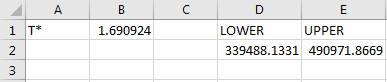
| tstar = t.ppf(1-0.5*0.13,42) |
Let’s name the lower value of the confidence interval as Lower. At the prompt, type the following to compute the lower value of the confidence interval and assign it to Lower.
| Lower = 621.63 - tstar*122.3/sqrt(43) |
Repeat the process for calculating the upper value of the confidence interval. Assign it to the name Upper.
| Upper = 621.63 + tstar*122.3/sqrt(43) |
Let’s have Python print out the confidence interval. Type the following.
| print "(%f, %f)" %(Lower, Upper) |
You should obtain the confidence interval . Figure 8.14 represents the layout you should have in Python when finished.
Comparing the confidence intervals with Examples 8.1.3 and 8.1.4 with those in Examples 8.1.7 and 8.1.8, you will notice that the confidence intervals in Examples 8.1.7 and 8.1.8 are wider. As mentioned before, estimating with means we need to account for more variability. So we expect wider confidence intervals whenever we use instead of .
8.1.3 Understanding the Confidence Interval
Interpreting a Confidence Interval
It is important to understand what the confidence interval is trying to describe to us. First and foremost, you should remove the following from your belief of what the confidence interval is.
The true mean is always within the range represented by the confidence interval.
This may not be true. Confidence intervals have a likelihood involved. In fact, the confidence level is the likelihood associated with the confidence interval.
Let’s get a better grasp of what is going on. Let’s create a confidence interval for , assuming the data we gather come from a normally distributed population. Assume further that is known and the sample size is fixed.
We have everything needed to start calculating the confidence interval for except for the sample mean. Well, that’s easy to obtain. We take a simple random sample from the normally distributed population and calculate a sample mean, call it . We have everything we need. So, we can go ahead and calculate a confidence interval for .
Meanwhile, a friend of ours from class also does the same thing. He or she takes a simple random sample from the population and calculates a sample mean, call it . Then they calculate a confidence interval for . (Note that their , ,, and are all the same.) Their confidence interval looks like
What’s the difference? Well, their will most likely be different than ours. So their confidence interval for will most likely be different. An argument ensues over which interval has in it. As a result, we both decide to repeat the process. We obtain a different sample mean, , and our obstinate friend gets a different sample mean, . Here are the different confidence intervals for .
These are different than our originals! Is there something wrong with the way the intervals are calculated? Nope! Remember that changes with each simple random sample collected from a population. If our friend and us each did this 50 times for a combined total of 100 different confidence intervals, then we should notice that some of the intervals may overlap. In fact, we should expect the proportion of of them to overlap. This is what the confidence interval is telling us.
For example, suppose that . Then if we were to construct one hundred confidence intervals for , 95 of them should contain the true population mean .
So, as a result, we should interpret the confidence interval for by stating the following.
We are confident that the confidence interval we obtained contains the population mean, .
In the statement, we are placing emphasis on the fact that there is a chance the confidence interval we obtained may not contain the population mean, . The above interpretation of a confidence interval for can be extended to the case of when we do not know . In fact, this same interpretation can be extended further to a confidence interval for any parameter, not just .
Changing : How a Confidence Intervals Changes
Based on this understanding of the confidence interval, your first thought may be, “Why not make as small as possible, say ?” This is a good question. The smaller is, the more likely a constructed confidence interval will capture the population mean, . However, there is a drawback to making be super small. The smaller gets, the range the confidence interval describes will widen. The best way to see this is through an example.
Example 8.1.9.
Let , , and . In Excel, calculate confidence intervals for given the following confidence levels.
-
1.
So . Using the command , we obtain . Calculating the confidence interval in the same manner as that in Example 8.1.3, we have
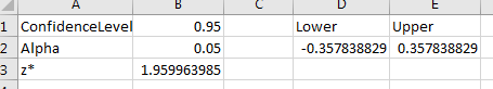
Figure 8.15: Excel Confidence Interval -
2.
So . Using the command , we obtain . Calculating the confidence interval, we have
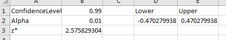
Figure 8.16: Excel Confidence Interval -
3.
So . Using the command , we obtain . Calculating the confidence interval, we have
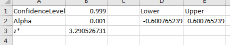
Figure 8.17: Excel Confidence Interval -
4.
So . Using the command , we obtain . Calculating the confidence interval, we have
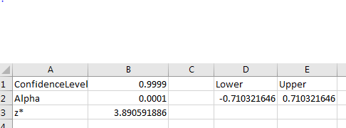
Figure 8.18: Excel Confidence Interval
Notice that as decreases, the confidence interval widens.
Ideally, we or will suffice. However, if targeting the population mean is important, there is another tactic we can take to try to shrink the confidence interval.
Controlling the Width of Confidence Interval through
While keeping is ideal, we can still adjust the confidence interval by adjusting the sample size . That will allow us to control the width of the sample size.
Recall that the confidence interval is sometimes written as
where or , depending on whether is known or not, this is called the margin of error for . The margin of error tells us how much we are allowed to deviate to the left and to the right of the sample mean when constructing the confidence interval for .
Say we want the margin of error to be not more than . That is, whenever we construct a confidence interval for we want the interval to look like
for some that was taken from a sample. How do we insure that the margin of error is or rather any other desired value of margin of error?
Since is assumed to be fixed and is given, the only other variable we can adjust is the sample size, . With a little algebra, we can obtain an expression that will tell us how big needs to be. In fact, by letting (or ), and (or ), and solving the formula
for , we have
This then gives us what we need.
Theorem (Controlling Margin of Error with ).
Given , and , in order to insure that the confidence interval for has a margin of error of at most , then the sample size, , needs to be at least
where (or ), and (or ), depending on whether we know or not.
Let’s see an example in Python for determining the appropriate sample size.
Example 8.1.10.
A quality controller wants to determine a 90% confidence interval for the average size of bolt manufactured. He knows that his population standard deviation is 1.2 mm and that he wants a margin of error of . How big must his sample sizes be in order to achieve his desired confidence intervals?
This question is really asking for the minimum sample size needed to ensure that the margin of error is at most . This is done by calculating the expression
Since we will be using Python, make sure you first load the following libraries before proceeding.
| from numpy import * |
| from scipy.stats import * |
First, we need to find . Since , then . In Python, type the following command will tell us . Store it as zstar.
| zstar = norm.ppf(1-0.5*0.1) |
We are given that and that we want a margin of error of . Since the expression for involves squaring, we do not need to worry about the as squaring will always return a non-negative value.
In Python, type the following to evaluate the expression for . Save it as n.
| n = (zstar*1.2/0.02)**2 |
Recall that squaring in Python will involve ** instead of a caret symbol.3535If done in Excel, you would use instead. Also notice that we do not need to worry about integer division since all values are floating-point.
Call the variable n. You should obtain . Figure 8.19 represents the output you should obtain in Python.
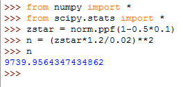
Since is an integer, we will round-up to the next whole integer. So, the quality controller should choose a sample size of at least 9740 to insure the margin of error is .
8.1.4 Exercises
-
1.
Answer each of the following statements as True or False.
-
(a)
The confidence intervals involving tend to be wider than the confidence intervals involving .
-
(b)
A confidence intervals for will always capture .
-
(c)
Making smaller will make the confidence interval wider.
-
(d)
There is a chance that the confidence interval you construct may not contain the population parameter.
-
(e)
The sample standard deviation can be used as an estimate of .
-
(a)
-
2.
Assuming normality in the population is satisfied, compute the confidence interval for in Excel given , , , and .
-
(a)
, , , .
-
(b)
, , , .
-
(c)
, , , .
-
(a)
-
3.
Assuming normality in the population is satisfied, compute the confidence interval for in Excel given , , , and .
-
(a)
, , , .
-
(b)
, , , .
-
(c)
, , , .
-
(a)
-
4.
Assuming normality in the population is satisfied, compute the confidence interval for in Python given , , , and .
-
(a)
, , , .
-
(b)
, , , .
-
(c)
, , , .
-
(a)
-
5.
Assuming normality in the population is satisfied, compute the confidence interval for in Excel given , , , and .
-
(a)
, , , .
-
(b)
, , , .
-
(c)
, , , .
-
(a)
-
6.
Given and , find the minimum sample size needed to obtain the stated margin of error, .
-
(a)
; , .
-
(b)
; , .
-
(c)
; , .
-
(a)
-
7.
Given , and , find the minimum sample size needed to obtain the stated margin of error, .
-
(a)
; , .
-
(b)
; , .
-
(c)
; , .
-
(a)
-
8.
Create an Excel worksheet that computes the confidence interval for for the case we know . It should be user friendly and only require the user to input , , , and .
-
9.
Create an Excel worksheet that computes the confidence interval for for the case we don’t know . It should be user friendly and only require the user to input , , , and .
-
10.
Create a script in Python that computes the confidence interval for for the case we know . The user should only be required to input , , , and .
-
11.
Create a script in Python that computes the confidence interval for for the case we don’t know . The user should only be required to input , , , and .