7 Population Models 7.4 The Uniform Distribution 7.6 The

t

7.5 The Normal Distribution

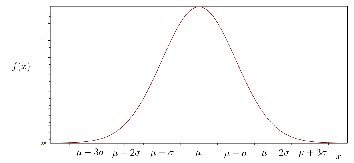
Carl Friedrich Gauss invented the normal distribution, perhaps the most important distribution in statistics. Here is a technical definition: a continuous random variable $X$ has a normal distribution with mean $\mu$ and standard deviation $\sigma$ if the p.d.f. is

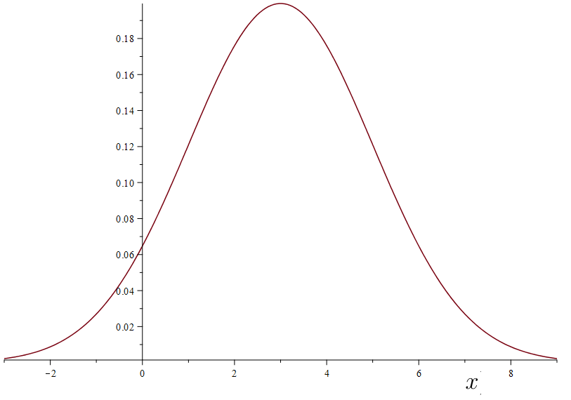
f(x)=\frac{1}{\sqrt{2\pi}\sigma}e^{\frac{-(x-\mu)^{2}}{2\sigma^{2}}},\qquad-% \infty<x<\infty.

Figure 7.10 gives a plot of the distribution.

Things to know:

1.

Our shorthand for “ $X$ is normally distributed with mean $\mu$ and standard deviation $\sigma$ ” will be $X\sim N(\mu,\sigma).$ So, for example, $X\sim N(3,8)$ means $X$ is normally distributed with mean $\mu=3$ and standard deviation $\sigma=8.$
2.

The distribution is symmetric and bell-shaped, and is centered at the mean $\mu.$ Thus, the mean locates the center of the distribution. The standard deviation $\sigma$ controls the spread of the distribution. The location and spread are illustrated in Figure 7.11.

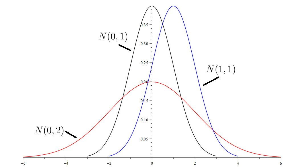
Figure 7.11: Different Normal Distributions
3.

The graph of $y=f(x)$ has exactly two inflection points. They are located horizontally at $\mu-\sigma$ and $\mu+\sigma,$ respectively.
4.

If $X\sim N(\mu,\sigma),$ then $P(X>\mu)=P(X<\mu)=0.5.$

Other then a few very special cases, it is not possible to compute exact areas under a normal distribution, making approximation techniques necessary. For our purposes, Excel has two built-in commands for working with a normal distribution that we will use frequently. They are covered in the next to sections.

7.5.1 Excel’s NORM.DIST

The Excel command NORM.DIST approximates areas for a normal distribution. Given $X\sim N(\mu,\sigma)$ and any real number $x,$ then

P(X<x)\approx\tt{\color{red}\colorlet{pgfstrokecolor}{.}\mbox{NORM.DIST}({\it x% },\mu,\sigma,\mbox{TRUE)}}

It’s vital to recognize that the command gives the area to the left of $x$ , as illustrated below.

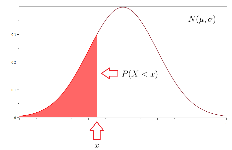
Figure 7.12: $P(X<x)\approx\tt{\color{red}\colorlet{pgfstrokecolor}{.}\mbox{NORM.DIST}({\it x% },\mu,\sigma,\mbox{TRUE)}}$

This means that if $X\sim N(\mu,\sigma)$ and if you want to approximate $P(X>x)$ using NORM.DIST, you must subtract the result of the command from 1, that is,

P(X>x)\approx\tt{\color{red}\colorlet{pgfstrokecolor}{.}\mbox{1 - NORM.DIST}({% \it x},\mu,\sigma,\mbox{TRUE)}}.

Similarly, if $a$ and $b$ are real numbers with $a<b,$ then

P(a<X<b)=P(X<b)-P(X<a),

and so

P(a<X<b)\approx\tt{\color{red}\colorlet{pgfstrokecolor}{.}\mbox{NORM.DIST}({% \it b},\mu,\sigma,\mbox{TRUE)}-\mbox{NORM.DIST}({\it a},\mu,\sigma,\mbox{TRUE)% }}.

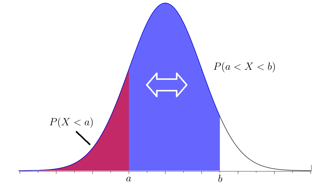
These computations are illustrated in the next example.

Example 7.5.1.

Suppose that $X\sim N(3,2),$ so that $X$ is normally distributed with mean $\mu=3$ and standard deviation $\sigma=2.$ A graph of the distribution is given below.

Some probability calculations in Excel:

1.

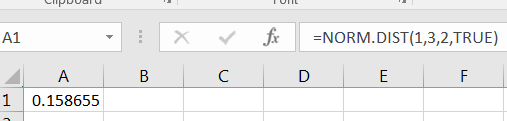
$P(X<1)\approx\tt{\color{red}\colorlet{pgfstrokecolor}{.}\mbox{NORM.DIST}(1,3,2% ,\mbox{TRUE)}}\approx 0.158655254$

Figure 7.15: Area to the Left of 1
2.

$P(X>1)\approx\tt{\color{red}\colorlet{pgfstrokecolor}{.}1-\mbox{NORM.DIST}(1,3% ,2,\mbox{TRUE)}}\approx 0.841344746$

Figure 7.16: Area to the Right of 1
3.

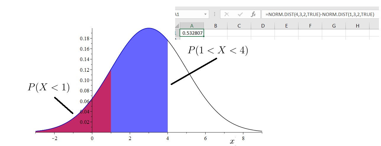
$\begin{array}[]{rcl}P(1<X<4)&=&P(X<4)-P(X<1)\\ &\approx&\tt{\color{red}\colorlet{pgfstrokecolor}{.}\mbox{NORM.DIST}(4,3,2,% \mbox{TRUE)}-\mbox{NORM.DIST}(1,3,2,\mbox{TRUE)}}\\ &\approx&0.532807207\\ \end{array}$

Figure 7.17: Area between 1 and 4

$\clubsuit$

7.5.2 Excel’s NORM.INV

Excel’s NORM.INV reverses the process of NORM.DIST. That is, where NORM.DIST computes an area to the left of a given value of $X,$ the command NORM.INV computes a value for $X$ for given area to the left. Suppose that $X\sim N(\mu,\sigma)$ and suppose that you want to find the value $x$ such that $P(X<x)=A,$ for some desired area $A$ . Then

x\approx\tt{\color{red}\colorlet{pgfstrokecolor}{.}\mbox{NORM.INV}({\it A},\mu% ,\sigma)}.

In other words, NORM.INV computes percentile scores of normal distributions. Following are some example computations.

Example 7.5.2.

Suppose again that $X\sim N(3,2).$

1.

The value $x$ where $P(X<x)=0.8$ is

$x\approx\tt{\color{red}\colorlet{pgfstrokecolor}{.}\mbox{NORM.INV}(0.8,3,2)}% \approx 4.683242467.$

Thus, the 80th percentile of $X$ is approximately 4.683242467.

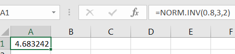
Figure 7.18: 80th Percentile of $X\sim N(3,2)$
2.

If we apply NORM.DIST to the prior result, we’ll get 0.8, demonstrating the relationship between NORM.DIST and NORM.INV.

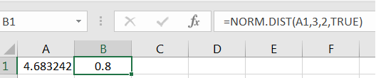
Figure 7.19: NORM.DIST and NORM.INV are Inverse Functions

$\clubsuit$

7.5.3 The Standard Normal Distribution

The normal distribution with mean 0 and standard deviation 1 is called the standard normal distribution. For the standard normal distribution, it is customary to use the letter $Z$ for the distribution, so $Z\sim N(0,1)$ is the shorthand notation. The standard normal distribution is displayed in Figure 7.11.

Suppose that $X\sim N(\mu,\sigma).$ It is a theorem of calculus that the random variable

\frac{X-\mu}{\sigma}

has a standard normal distribution,³⁰³⁰Recall that if a population $X$ has mean $\mu$ and standard deviation $\sigma,$ then $\frac{x-\mu}{\sigma}$ gives the number of standard deviations $x$ is from $\mu.$ i.e.,

Z=\frac{X-\mu}{\sigma}.

Moreover, for any two real numbers $a$ and $b,$ with $a<b,$ from calculus it can be shown that

P(a<X<b)=P\left(\frac{a-\mu}{\sigma}<Z<\frac{b-\mu}{\sigma}\right).

(7.5)

Equation (7.5) allows for computing areas for any normal distribution by computing areas using only the standard normal, which is of computational significance if one doesn’t have access to command like NORM.DIST or NORM.INV. The following example illustrates.

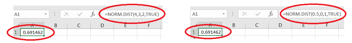
Example 7.5.3.

Suppose again that $X\sim N(3,2).$ Note that the value $x=4$ is 0.5 standard deviations above the mean. This means that the area to the left of 4 in $N(3,2)$ is the same as the areas to the left of 0.5 in $N(0,1).$ See Figure 7.20.

Figure 7.20: Equal Areas Under Different Normal Distributions

$\clubsuit$

7.5.4 The 68 - 95 - 99.7 “Rule”

Suppose that $X$ is a random variable with mean $\mu$ and standard deviation $\sigma.$ Recall that the phrase “ $x$ is within $k$ standard deviations of the mean” means that $x$ satisfies the inequality

\mu-k\sigma\leq x\leq\mu+k\sigma,

or that $x$ is in the interval $[\mu-k\sigma,\mu+k\sigma].$ Knowing

P(\mu-k\sigma\leq X\leq\mu+k\sigma)

for various values of $k$ provides information on the behavior of the random variable $X .$

Suppose that $X\sim N(\mu,\sigma)$ and let $k$ be a positive integer. Equation (7.5) gives that the probability a randomly generated $X$ is within $k$ standard deviations of the mean is the same as the probability that a randomly generate number from a standard normal distribution is within the interval $(-k,k).$ That is,

P(\mu-k\sigma<X<\mu+k\sigma)=P(-k<Z<k).

So, for a normally distributed population $X\sim N(\mu,\sigma),$ the proportion of that falls within 1 standard deviation of the mean is

\begin{array}[]{rcl}P(\mu-\sigma\leq X\leq\mu+\sigma)&=&P(-1<Z<1)\\ &\approx&\tt{\color{red}\colorlet{pgfstrokecolor}{.}\mbox{NORM.DIST}(1,0,1,% \mbox{TRUE)}-}\\ &&\qquad\tt{\color{red}\colorlet{pgfstrokecolor}{.}\mbox{NORM.DIST}(-1,0,1,% \mbox{TRUE)}}\\ &\approx&0.682689492\end{array}

In words, for a normally distributed population, about 68.3% of all values fall within 1 standard deviation of the mean.

Similarly, again for $X\sim N(\mu,\sigma),$ the proportion that fall within 2 standard deviations of the mean is

\begin{array}[]{rcl}P(\mu-2\sigma\leq X\leq\mu+2\sigma)&=&P(-2<Z<2)\\ &\approx&\tt{\color{red}\colorlet{pgfstrokecolor}{.}\mbox{NORM.DIST}(2,0,1,% \mbox{TRUE)}-}\\ &&\qquad\tt{\color{red}\colorlet{pgfstrokecolor}{.}\mbox{NORM.DIST}(-2,0,1,% \mbox{TRUE)}}\\ &\approx&0.954499736\end{array}

Thus, for a normally distributed population, about 95% of all values fall within 2 standard deviations of the mean.

The reader should check that for a normally distributed population, the percent that fall within 3 standard deviations of the mean is about 99.7%. Combining these results is typically called the “The 68 - 95 - 99.7 Rule.” The choice of word “rule” is unfortunate, as this isn’t a rule, but instead is a theorem. Theorems are not arbitrary diktats, but instead are true statements backed by rigorous proofs. This text isn’t concerned with rigorous mathematical proofs, but know that they exist.

A word of caution on the 68 - 95 - 99.7 rule: this holds for normally distributed populations. If you are working with a population that has a different distribution, then these percents a likely different.

7.5.5 Central Limit Theorem

We now discuss one of the most important theorems in statistics, which ultimately in the punchline of the prior chapter. Recall that whether looking at sample means or sample proportions, their distributions were roughly bell-shaped and symmetric, centered at the mean of the population from which the samples were taken. Moreover, as the sample size increased, the spread of the sample means and sample proportions shrunk. This behavior can be proved, and is known as the Central Limit Theorem (CLT).

Theorem (The Central Limit Theorem). Suppose that a large population $X$ has mean $\mu$ and finite standard deviation $\sigma.$ For random samples of size $n,$ if $n$ is sufficiently large, then the distribution for $\bar{X}$ will be approximately normal, with the mean approximately $\mu,$ and standard deviation approximately $\sigma/\sqrt{n}.$ In symbols, $\bar{X}\sim N(\mu,\sigma/\sqrt{n}).$ One can also write $\mu_{\bar{X}}\approx\mu$ and $\sigma_{\bar{X}}\approx\sigma/\sqrt{n}.$

Remarks:

•

If the population $X\sim N(\mu,\sigma),$ then for any sample size $n,$ $\bar{X}\sim N(\mu,\sigma/\sqrt{n}),$ i.e., if $X$ is normal, $\bar{X}$ is always normal with mean $\mu$ and standard deviation $\sigma/\sqrt{n}.$
•

If $X$ is “pathological,” large sample sizes may be necessary to see bell-shaped distributions for $\bar{X}.$ For our purposes, we will use $n\geq 30$ as a rule-of-thumb for sufficiently large.
•

Note that the standard deviation of $\bar{X}$ gets smaller as $n$ gets larger.

Example 7.5.4.

Suppose population $X$ has mean $\mu=4$ and standard deviation $\sigma=7.$ Suppose a random sample size $n=30$ is drawn from the population. Estimate $P(\bar{X}>5).$ ³¹³¹In words, if a random sample of size 30 is drawn from a population with mean 4 and standard deviation 7, what is the probability that the sample mean is greater than 5.

Solution: Since $n=30,$ we can use CLT. Now $\mu_{\bar{X}}\approx 4$ and $\sigma_{\bar{X}}\approx 7/\sqrt{30}.$ Since the distribution of $\bar{X}$ is approximately normal, using Excel we have

P(\bar{X}>5)\approx\tt{\color{red}\colorlet{pgfstrokecolor}{.}1-\mbox{NORM.% DIST}(5,4,7/SQRT(30),\mbox{TRUE)}}\approx 0.2170.

$\clubsuit$

When working with proportions, the CLT still applies, but the notation is changed a bit.

Corollary Suppose that a large population contains a proportion $p$ of things of Type A. For random samples of size $n,$ if $n$ is sufficiently large, then the distribution of sample proportions $\hat{P}$ of things of Type A will be approximately normal, with the mean approximately $p,$ and standard deviation approximately $\sqrt{p(1-p)/n}.$ In symbols, $\hat{P}\sim N(p,\sqrt{p(1-p)/n}.$ One can also write $\mu_{\hat{P}}\approx p$ and $\sigma_{\hat{P}}\approx\sqrt{p(1-p)/n}.$

Remark:

•

If population is “pathological,” large sample sizes may be necessary to see bell-shaped distributions for $\hat{P}.$ For our purposes, we will use $np\geq 10$ and $n(1-p)\geq 10$ as a rule-of-thumb for sufficiently large.

Example 7.5.5.

Suppose a population contains $p=0.3$ things of Type A. Suppose a random sample size $n=100$ is drawn from the population. Estimate $P(\hat{P}<0.25).$ ³²³²In words, if a random sample of size 100 is drawn from a population with $p=0.3,$ what is the probability that the sample proportion is smaller than 0.25.

Solution: Since $np=100\cdot 0.3=30\geq 10$ and $n(1-p)=70,$ we can use CLT. Now $\hat{P}\sim N(0.3,\sqrt{0.3\cdot 0.7/100}),$ using Excel we have

P(\hat{P}<0.25)\approx\tt{\color{red}\colorlet{pgfstrokecolor}{.}\mbox{NORM.% DIST}(0.25,0.3,SQRT(0.3*0.7/100),\mbox{TRUE)}}\approx 0.1376.

$\clubsuit$

7.5.6 CLT Simulation - Optional

In the prior chapter, we saw several demonstrations that sample means and sample proportions have approximately bell-shaped distributions centered at the population mean or proportion, respectively. Let’s do that again, while checking on the mean and standard deviation of sample statistics.

The simulation will be sharpest if we make the population normal, so let us use

X\sim N(5,2).

The sample size doesn’t matter, so we’ll use $n=10$ here. Thus, in this simulation, we will have

\bar{X}\sim N(5,2/\sqrt{10}).

(7.6)

Use Excel to simulate taking 1,000 samples of size 10 from $X\sim N(5,2).$

We’ll compare the observed behavior of the sample means to (7.6). For each sample, compute $\bar{x},$ and then create a frequency histogram for the 1,000 sample means. You’ll get a histogram that looks similar to Figure 7.22.

Note the bell shape, and that the mean of the $\bar{x}$ ’s appears to be about 5. Compute the sample mean and sample standard deviation of the sample means, as in Figure 7.23.

Figure 7.23: Statistics of the $\bar{x}$ ’s

Your sample mean of the sample means will be close to 5. Moreover, your sample standard deviation of the sample means will be near to $2/\sqrt{10}\approx 0.6325.$

Lastly, compute the percent of $\bar{x}$ ’s that fall within 1, 2 and 3 standard deviations of the mean. You’ll get results that are very close to the 68-95-99.7 rule for normal populations. First compute the bounds of the three intervals about the mean of the sample means, as in Figure 7.24.

Figure 7.24: Intervals about the Sample Mean of the $\bar{x}$ ’s

Then count the number of $\bar{x}$ ’s that fall to the left of the lower and upper bounds of the intervals, as in Figure 7.25.

Now the percents can be computed directly, as in Figure 7.26. The results will give further evidence that the sample means have a normal distribution.

7.5.7 Exercises

1.

Suppose that $X\sim N(3,5).$ Find the mean $\mu$ and standard deviation $\sigma$ of $X,$ compute $P(X<4),$ $P(X>4),$ and $P(2<X<4),$ and sketch each probability.
2.

Compute $P(Z<1.5),$ $P(Z>-1.5),$ and $P(-1.5<Z<1.5).$ Sketch each probability.
3.

Suppose that $X\sim N(3,5).$ Compute the first and third quartiles of $X .$
4.

For a certain standardized exam, scores $X$ are normally distributed with a mean of 100 and standard deviation of 10. What exam score is needed to be above the 90th percentile?
5.

Compute $z>0$ such that $P(-z<Z<z)=0.95.$ Sketch a picture that illustrates.
6.

Suppose population $X$ has mean 6 and standard deviation 10. A random sample of size 100 is drawn from $X .$ Estimate $P(5<\bar{X}<7).$
7.

Suppose population $X$ has mean 8 and standard deviation 4. A random sample of size 40 is drawn from $X .$ Estimate $P(\bar{X}>9).$
8.

A random sample of size 8 is drawn from $X\sim N(-4,3).$ Compute $P(\bar{X}<-3).$
9.

At a large school, 65% of students participate in athletics. A random sample of 200 students is drawn. What is the probability that the observed sample percentage of athletes is greater than 70%?
10.

A fair 6-sided die is rolled 300 times, and the proportion of 1’s observed is recorded. Approximate the probability that the proportion of observed 1’s exceeds 0.2.
11.

Suppose that $X\sim N(10,5),$ and suppose that a random sample of size 50 is drawn from $X .$ Compare the values of $P(X>11)$ and $\bar{X}>11).$
12.

(Optional) Let $X\sim U(0,12).$ We know that $\mu=6,$ and it turns out that $\sigma=12.$ Use a simulation to study the behavior of $\bar{X}$ for samples of size 50. Compare the results to the CLT.