7.4 The Uniform Distribution
For purposes of computing probabilities with ease, the uniform distribution is handy. Suppose that is a continuous random variable with p.d.f. We say has a uniform distribution if there are real numbers and with such that
We say that is uniformly distributed between and and our shorthand notation for this distribution will be
Notes:
-
•
In graphing the uniform distribution, over the interval draw a rectangle of height as shown in Figure 7.7.
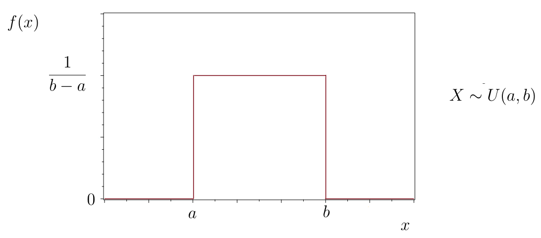
Figure 7.7: Uniform Distribution U(a,b) -
•
If an is randomly generated, it will be between and i.e., it won’t be less than or greater than
-
•
Since the total area must be 1, the height of the box is
-
•
By symmetry, the mean of is the midpoint of the interval i.e., it is the average of the two endpoints. In symbols,
Knowing this is handy in interpreting some simulations.2929It turns out that if then the variance of is This too can be handy for some simulations.
-
•
Computing probabilities amounts to computing areas of rectangular boxes, as illustrated in the next example.
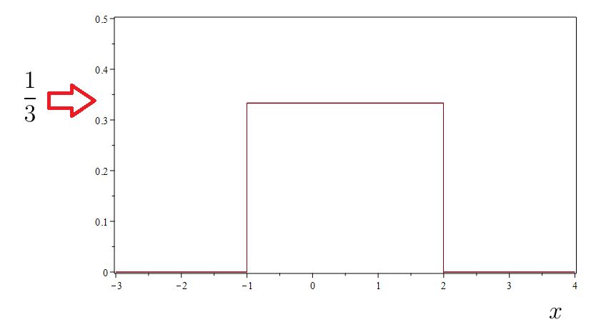
Example 7.4.1.
Suppose The graph of the p.d.f. is shown in Figure 7.8.
To illustrate computing probabilities, let’s compute The area is illustrated in Figure 7.9.
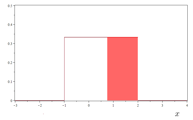
The width of the box is while the height of the box is 1/3. Thus,
Note that the mean of is
Exercises
-
1.
Suppose Sketch the distribution, labeling the axes appropriately, sketch and compute and compute the mean of
-
2.
Suppose Sketch the distribution, labeling the axes appropriately, sketch and compute and compute the mean of