7 Population Models 7.2 Discrete Random Variables 7.4 The Uniform Distribution

7.3 Continuous Random Variables

If the random variable $X$ is continuous, then probabilities for observed values of $X$ are described differently than the discrete case. In the continuous case, $X$ is accompanied by a probability density function (p.d.f.) $f(x).$ To be a proper p.d.f., the function $f(x)$ must satisfy the following:²⁸²⁸Equation 7.4 uses calculus. If you’ve not had calculus, ignore the symbols, and focus on the verbal description.

•

For all $-\infty<x<\infty,$ $f(x)\geq 0.$
•

For any $a$ and $b$ with $a<b,$ the probability that a randomly generated $X$ is between $a$ and $b$ is the area under the graph of $y=f(x),$ i.e.,

$P(a<X<b)=\int_{a}^{b}f(x)\,dx.$ (7.4)
•

The total area under the graph of $y=f(x)$ is 1, that is,

$\int_{-\infty}^{\infty}f(x)\,dx=1$

Notes:

•

Figure 7.6 gives a graphical representation of $P(a<X<b).$

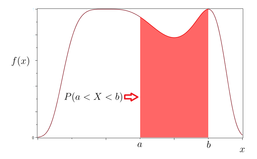
Figure 7.6: Area Under Curve as $P(a<X<b)$
•

For any real number $a,$ $P(X=a)=0,$ because the area of a line segment is 0. This may seem odd, but it’s the nature of the beast. It follows as well that $P(X\leq a)=P(X<a).$