7 Population Models 7.1 Populations and Random Variables 7.3 Continuous Random Variables

7.2 Discrete Random Variables

If the possible values of a random variable $X$ are discrete, then the $X$ is a discrete random variable. The populations in Examples 6.2.1, 6.2.2, and 6.2.2 are all discrete.

If the values possible values of a discrete random variable $X$ are $x_{1},x_{2},x_{3},\ldots,$ then we will write

X=\left\{x_{1},x_{2},x_{3},\ldots\right\}.

For example, if $X$ is the outcome of rolling a standard 6-sided die, then we could write $X=\left\{1,2,3,4,5,6\right\}.$ The notation $X=2$ would denote the event that the outcome of a roll is 2.

With a discrete random variable $X$ the manner in which probabilities of outcomes is described works as follows: for each possible value $x$ of $X,$ the probability of observing $X=x$ is denoted by $p_{x},$ i.e.,

P(X=x)=p_{x}.

(7.1)

The function in Equation 7.1 is called a probability mass function (pmf), and Equation 7.1 can be read as “the probability of observing the value $x$ is $p_{x}.$ ”

For the function to be a proper pmf, the following must hold:

•

For each possible value $x$ of $X,$ $p_{x}\geq 0.$
•

The sum of all of the probabilities must be exactly 1, i.e., if $X=\left\{x_{1},x_{2},x_{3},\ldots\right\},$ then

$p_{x_{1}}+p_{x_{2}}+p_{x_{3}}+\cdots=1.$

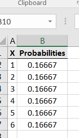
For example, suppose $X$ is the outcome of rolling a fair 6-sided die. Then $P(X=1)=1/6,$ $P(X=2)=1/6,$ etc. Discrete random variables and their corresponding pmf’s can be displayed nicely with a table. With this $X,$ for example, this table completely describes the random variable:

X	P(X=x)
1	1/6
2	1/6
3	1/6
4	1/6
5	1/6
6	1/6

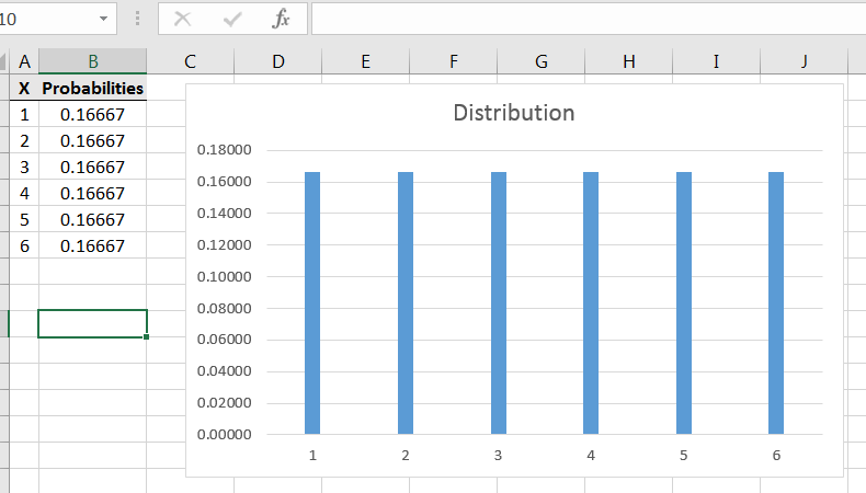
Additionally, a discrete random variable distribution can be graphed as follows: at each location $x_{i}$ along the horizontal axis, draw a stick with height equal to $p_{x_{i}}.$ In Excel, the table and graph will could look like Figure 7.1.

Lastly, the probability notation introduced is handy. For example, suppose $X$ is the outcome of rolling a fair 6-sided die. The symbol $P(X\leq 3)$ denotes the probability that a roll results in a 3 or less, i.e., it is the probability of rolling a 1, 2, or 3. In this case, we would have

P(X\leq 3)=P(X=1)+P(X=2)+P(X=3)=\frac{1}{6}+\frac{1}{6}+\frac{1}{6}=\frac{1}{2}.

Concepts Check 1. A fair coin is flipped 4 times, and let

X

be the proportion of heads observed. What are the possible values of

X ?

Answer:

X=\{0,1/4,1/2,3/4,1\}

2. A fair 4-sided die has faces marked as 1, 3, 7 and 9, respectively. Let

X

be the outcome of a single roll of the die. What is

P(X=9)=?

Answer: 1/4 3. Using

X=\left\{1,3,7,9\right\}

in the prior problem, compute

P(X>3).

Answer: 1/2

7.2.1 Exercises

1.

A fair coin is flipped 4 times, and let $X$ be the proportion of heads observed. Use a simulation to estimate $P(X=3).$
2.

A fair 4-sided die has faces marked as 1, 3, 7 and 9, respectively. Let $X$ denote the outcome of a single roll. In Excel, enter the distribution of $X$ as a table, and then create a graph that displays the distribution.
3.

A fair 4-sided die has faces marked as 1, 3, 7 and 9, respectively. The die is rolled twice, and $X$ represents the sum of the two rolls. Use a simulation to estimate $P(X\leq 3).$

7.2.2 Mean of a Discrete Random Variable - Optional

We will use discrete random variables principally for simulating taking samples from known populations. However, if you are studying a discrete random variable and if you happen to know exactly the corresponding pmf, then you can calculate the mean $\mu$ of the population as follows. Suppose $X=\left\{x_{1},x_{2},x_{3},\ldots\right\}$ and $P(X=x)=p_{x}.$ Then

\mu=\sum_{i=1}^{\infty}x_{i}\cdot p_{x_{i}}=x_{1}\cdot p_{x_{1}}+x_{2}\cdot p_% {x_{2}}+x_{3}\cdot p_{x_{3}}+\cdots

(7.2)

In words, here’s what you do: for each possible value $x,$ multiply it by its corresponding probability $p_{x},$ and then add up all of those products. That gives the mean $\mu.$ ²⁷²⁷If the number of possible values of $X$ is infinite, then the sum 7.2 (and hence the mean) might not exist. Tackling infinite sums is a problem introduced in calculus.

Example 7.2.1.

Consider the discrete random variable $X$ which is the outcome of rolling a fair 6-sided die:

Figure 7.2: Discrete Random Variable $X$

To compute $\mu,$ for each $x$ compute $x\cdot p_{x}$ in the adjacent column:

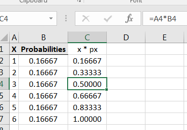
Then compute the sum of the entries:

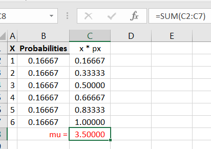
As expected, the average roll of a fair 6-sided die is 3.5. $\clubsuit$

The upshot is that there are a number of simulations in this text where you can calculate the exact value of a population mean $\mu$ directly, namely those that use a random variable that has only finitely many values.

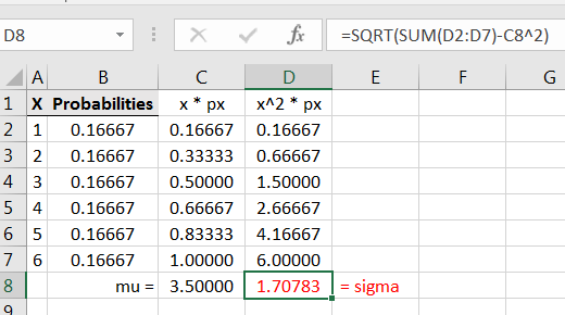
7.2.3 Standard Deviation of a Discrete Random Variable - Optional

The variance $\sigma^{2}$ of a discrete random variable is computed similarly. The most computationally friendly formula is follows. If random variable $X=\left\{x_{1},x_{2},x_{3},\ldots\right\}$ has pmf $P(X=x)=p_{x},$ then

\sigma^{2}=\left(\sum_{i=1}^{\infty}x_{i}^{2}\cdot p_{x_{i}}\right)-\mu^{2}=(x% _{1}^{2}\cdot p_{x_{1}}+x_{2}^{2}\cdot p_{x_{2}}+x_{3}^{2}\cdot p_{x_{3}}+% \cdots)-\mu^{2}

(7.3)

Taking the square-root of Equation 7.3 gives the standard deviation.

The calculation is demonstrated in Figure 7.3.