3 Summary Statistics in Excel 3 Summary Statistics in Excel 3.2 Displaying the Data

3.1 Excel Essentials

In this section, we’ll quickly run through how to manipulate Excel into doing computations for us.

Goals:

\bullet

Learn how to do arithmetic in Excel;

\bullet

Learn how to manipulate Excel to produce functions with Excel’s

Cell-Referencing;

\bullet

Be able to generate random numbers and create samples of data.

3.1.1 Arithmetic

Excel can be thought of as one big fancy calculator. At the bare minimum, Excel will do the same calculations that a common calculator will do. There is much more to the software can do than just a common calculator, of course.

Basic Operations

In the table below, you will find the five main operations that are typically found on any standard calculator: addition, subtraction, multiplication and division. Along with each, the syntax to implement the operation in Excel is no different that what one may expect.

Addition	$+$
Subtraction	$\tt{\color{red}\colorlet{pgfstrokecolor}{.}-}$
Multiplication	$\tt{\color{red}\colorlet{pgfstrokecolor}{.}*}$
Division	$\tt{\color{red}\colorlet{pgfstrokecolor}{.}/}$
Powers	$\wedge$

Figure 3.1: Excel Operations

From here on out, commands done in Excel will highlighted in red. To perform arithmetic in Excel, an equal sign, $\tt{\color{red}\colorlet{pgfstrokecolor}{.}=}$ is required. Let’s try out an example.

Example 3.1.1.

Let’s compute the expression

\dfrac{(2.9-2.4)^{2}+(3.1-2.4)^{2}+(4.0-2.4)^{2}+(1.1-2.4)^{2}+(0.9-2.4)^{2}}{% 4}.

In any cell in Excel, type the following:

\tt{\color{red}\colorlet{pgfstrokecolor}{.}=((2.9-2.4)\wedge 2+(3.1-2.4)\wedge 2% +(4.0-2.4)\wedge 2+(1.1-2.4)\wedge 2+(0.9-2.4)\wedge 2)/4}

Once you typed it in, press the enter key. Excel will output the solution $\tt{\color{red}\colorlet{pgfstrokecolor}{.}1.81}$ . $\clubsuit$

You should be aware of the importance of the parentheses when entering in the expression in Figure 3.2. Computers rely on order of operations, the same concept taught in any algebra course. Dropping parentheses may incorrectly calculate the expression.

Square Root, Exponentials, Trigonometric, and Logarithmic Functions

Excel is capable of performing many other mathematical functions. However, these involve typing a command. Below is a table that summarizes such functions.

Square Root	SQRT(…)
Exponential Function	EXP(…)
Sine Function	SIN(…)
Cosine Function	COS(…)
Logarithm (base 10)	LOG(…)
Logarithm (base $e$ )	LN(…)

Figure 3.3: Excel Nonlinear Operations

Ellipses in the commands denote input values from the user. All functions will return values as long as the inputted value is within the domain of the function. Be aware that the trigonometric functions require the input to be in radians instead of degrees.

Example 3.1.2.

Let’s compute the expression

\sin\left(\cos\left(\sqrt{\log{(10)}+e^{\ln{2}}}\right)\right).

In any cell, type the following:

\tt{\color{red}\colorlet{pgfstrokecolor}{.}=SIN(COS(SQRT(LOG(10)+EXP(LN(2)))))}

After hitting enter, you should obtain the answer $\tt{\color{red}\colorlet{pgfstrokecolor}{.}-0.159867612}$ . $\clubsuit$

Excel is useful in manipulating arrays of data. In fact, when implementing commands such as those in Figure 3.4, we often will select other cells as our input values. This is known as cell referencing. It is a novel way of constructing functions, mappings that produce well-defined output for some given input, of our own with inputs being specific cell ranges. Let’s repeat the previous example using cell-referencing in Excel.

Example 3.1.3.

Let’s compute the expression

\dfrac{(2.9-2.4)^{2}+(3.1-2.4)^{2}+(4.0-2.4)^{2}+(1.1-2.4)^{2}+(0.9-2.4)^{2}}{4}

using Excel’s cell referencing.

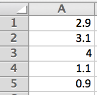
Begin by entering the data $\tt{\color{red}\colorlet{pgfstrokecolor}{.}2.9,3.1,4.0,1.1,0.9}$ into cells $\tt{\color{red}\colorlet{pgfstrokecolor}{.}A1}$ through $\tt{\color{red}\colorlet{pgfstrokecolor}{.}A5}$ in Excel.

Noticing that the value $\tt{\color{red}\colorlet{pgfstrokecolor}{.}2.4}$ shows up in each of the parentheses, input it into cell $\tt{\color{red}\colorlet{pgfstrokecolor}{.}B1}$ . We can now type the expression we wish to be calculated by calling the cells that our data is contained within. In cell $\tt{\color{red}\colorlet{pgfstrokecolor}{.}C1}$ , type the following:

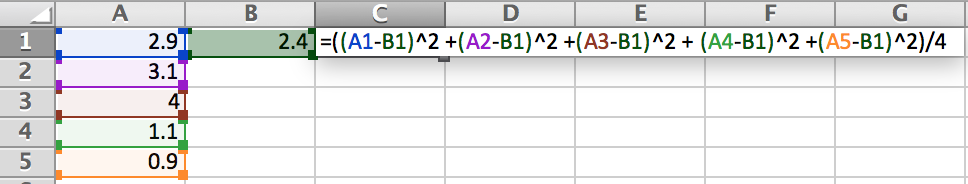
\tt{\color{red}\colorlet{pgfstrokecolor}{.}=((A1-B1)\wedge 2+(A2-B1)\wedge 2+(% A3-B1)\wedge 2+(A4-B1)\wedge 2+(A5-B1)\wedge 2)/4}

After entering the expression, we arrive at the same answer as that in the previous example: $\tt{\color{red}\colorlet{pgfstrokecolor}{.}1.81}$ . $\clubsuit$

It may seem as though the previous example is a lot more work than necessary. While this may be true at first, it is not always the case. In fact, by changing the values in cells $\tt{\color{red}\colorlet{pgfstrokecolor}{.}A1}$ – $\tt{\color{red}\colorlet{pgfstrokecolor}{.}A5}$ in the prevous example Excel will automatically do the calculations and update cell $\tt{\color{red}\colorlet{pgfstrokecolor}{.}C1}$ .

Expressions can be repeated over and over again. The next example demonstrates this.

Example 3.1.4.

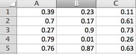
For each of the columns of data in the table below, add them up and then divide by the number of data values there are in each column.

0.39	0.23	0.11
0.7	0.17	0.61
0.27	0.9	0.73
0.79	0.01	0.26
0.76	0.87	0.63

On a new sheet, enter the data into columns $\tt{\color{red}\colorlet{pgfstrokecolor}{.}A}$ through $\tt{\color{red}\colorlet{pgfstrokecolor}{.}C}$ in Excel.

In cell $\tt{\color{red}\colorlet{pgfstrokecolor}{.}A7}$ , type the following and press enter:

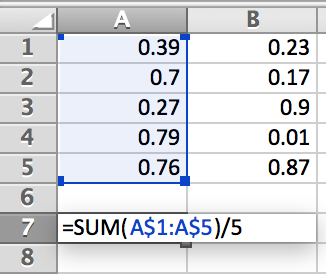
\tt{\color{red}\colorlet{pgfstrokecolor}{.}=SUM(A\$1:A\$5)/5}

Without having to retype the expression twice-over, we can click and drag the small rectangle in the lower right-hand corner of cell $\tt{\color{red}\colorlet{pgfstrokecolor}{.}A7}$ towards the right, ending on cell $\tt{\color{red}\colorlet{pgfstrokecolor}{.}C7}$ . Letting go of the drag will automatically calculate the expression for each column.

$\clubsuit$

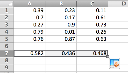
Notice that in this example, a couple shortcuts were implemented. One is the command $\tt{\color{red}\colorlet{pgfstrokecolor}{.}SUM(\ldots)}$ . This is shortcut for adding up the data in specified cells. The other is the auto-fill feature in Excel. It allowed us to quickly evaluate the same expression across several columns of data. This feature will be used quite a bit throughout the book.

It is also important to note the $\$$ used in Figure 3.9. This is used to tell Excel to hold cell indices. In this particular case, we wanted to hold the rows the same and allow the columns to change. Clicking on any of the cells in row 7 will show that the expression iterated over the columns and left the row indices the same. This technique will also be used quite a bit throughout the book.

3.1.2 Sampling Data

Statistics relies on sampling from a population in order to gain an understanding of the properties that the population may have.

Definition (Sample and Population).

The population is a complete collection of items that all share at least one characteristic, described by a variable name. A Sample is a nonempty subset taken from a population that is used as a representation of the population.

Ideally, we’d like to have the data encompass the entire population. However, this may be impossible to achieve. For example, if a manufacturing company wants to determine if the size of the bolts are being accurately made, it would be impractical to measure every single bolt produced. Time and money would be lost. The population in this case would be all of the bolts produced by the company. A sample of this population would be more ideal since it’s a snapshot of the entire population.

Simulations are done by generating samples of data from a population. A way of generating data is through the use of a random number generator. We have encountered random number generators in our day to day lives. Being asked, pick an integer between 1 and 10, then involves doing exactly what a random number generator does. When we are asked to pick a number, however, we tend to introduce biasness. To overcome this, we allow computers to randomly generate values based on certain criteria, i.e., an integer that is selected between 1 and 10 so that each number is equally likely to be selected. Let’s look at two commands in Excel that will help us create samples of data from a population by generating random numbers: $\tt{\color{red}\colorlet{pgfstrokecolor}{.}RAND()}$ and $\tt{\color{red}\colorlet{pgfstrokecolor}{.}RANDBETWEEN(A,B)}$ .

Rand() and Randbetween(a,b)

The command $\tt{\color{red}\colorlet{pgfstrokecolor}{.}RAND()}$ will generate a random number between 0 and 1, where every number between 0 and 1 are equally likely to be selected. We tend to use this when we know our data is allowed to take on values in a continuous nature.

Definition (Quantitative Continuous Variable).

Numerical variable that is allowed to take on any number within an interval of the real number line.

Here are several variables that are considered to be continuous, along with possible range of outputs that you may encounter from each which we could use $\tt{\color{red}\colorlet{pgfstrokecolor}{.}RAND()}$ to generate. Note: Interval notation is used to show possible ranges.

Measured Size of Feet (in inches)	$(0,17]$
100m Relay Times	$(0,\infty)$
Temperatures (in Celsius)	$[-273.15,\infty)$
Amount of Water (in gallons) Flowing Through Dam in a Day	$(0,\infty)$

Figure 3.10: Examples of Quantitative Continuous Variables

Let’s see how we can use $\tt{\color{red}\colorlet{pgfstrokecolor}{.}RAND()}$ to create sample of data that represents the number of a bacteria over a period of time.

Example 3.1.5.

The amount of cells present of a fast growing bacteria strain can be modeled using the logistic equation

P(t)=\dfrac{20}{1+3e^{-2t}},

where $P$ is measured in millions of cells and $t$ is time from 0 seconds 1 second. Let’s use the $\tt{\color{red}\colorlet{pgfstrokecolor}{.}RAND()}$ command in Excel to generate 10 populations at random time values between 0 and 1 second.

Starting a new sheet in Excel, type in cell $\tt{\color{red}\colorlet{pgfstrokecolor}{.}A1}$ the expression

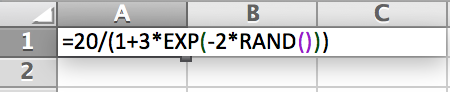
\tt{\color{red}\colorlet{pgfstrokecolor}{.}=20/(1+3*EXP(-2*RAND()))}

Figure 3.11: Using $\tt{\color{red}\colorlet{pgfstrokecolor}{.}RAND()}$

Pressing enter, a random population will be produced. Using Excel’s auto-fill feature, click and drag the lower right square down 9 more cells. This will produce the 10 randomly generated population values taken at 10 different times between 0 and 1 second.

$\clubsuit$

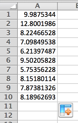
Remark: The values that you obtain will be different than those in Figure 3.12. Why is this?

The command $\tt{\color{red}\colorlet{pgfstrokecolor}{.}RANDBETWEEN(A,B)}$ is a little different than the $\tt{\color{red}\colorlet{pgfstrokecolor}{.}RAND()}$ command. In fact, $\tt{\color{red}\colorlet{pgfstrokecolor}{.}RANDBETWEEN(A,B)}$ generates a random integer between $a$ and $b$ . This is useful when we only need data values to take on integers within a specific range of numbers. That is, it is useful when we want to generate data that is discrete in nature.

Definition (Quantitative Discrete Variable).

A numerical variable that only takes on a finite number or countable number of possible values.

Here are several variables that are considered to be discrete, along with possible outputs, that $\tt{\color{red}\colorlet{pgfstrokecolor}{.}RANDBETWEEN(A,B)}$ could be used to generate samples of data.

Shoe Size	…, 6in, 6.5in, 7in, 7.5in, …, 10in, 10.5in, 11in, …
Number of Blue M&M‘s in a Bag	0, 1, 2, …, 25 …
Number of Students in a Class	0, 1, 2, …, 25 …
Sizes of Standard Wrenches Used	…, 1/2in, 9/16in, 5/8in, 11/16in, 3/4in, …

Figure 3.13: Examples of Quantitative Discrete Variables

Example 3.1.6.

All the days of the year are possible birthdays for a class. Assuming leap year is not an option, let’s create a sample of data from a class of 25 that represent the birthdays of each of the students in the class.

Not considering leap year, there are 365 possible values that could be potential birthdays. We can then randomly generate a number between 1 and 365 using a random number generator. Starting a new sheet in Excel, type in cell $\tt{\color{red}\colorlet{pgfstrokecolor}{.}A1}$ the expression

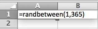
\tt{\color{red}\colorlet{pgfstrokecolor}{.}=RANDBETWEEN(1,365)}

Figure 3.14: $\tt{\color{red}\colorlet{pgfstrokecolor}{.}RANDBETWEEN(A,B)}$ Command

Pressing enter, we can then use Excel’s auto-fill feature to generate a random birthday 25 times. Click and drag the small rectangle in the lower right-hand corner of cell $\tt{\color{red}\colorlet{pgfstrokecolor}{.}A1}$ down until you reach row 25.

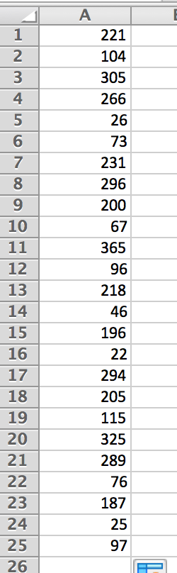
This sample then represents a class of 25 students’ birthdays. Be aware that the sample in Figure 3.15 will not be the same as what you obtain. $\clubsuit$

Data Analysis Toolpak: Random Number Generation

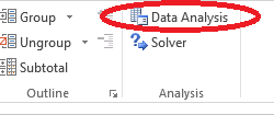
In Excel, locate the button Data Analysis within the ribbon tab DATA, as seen in Figure 3.16.

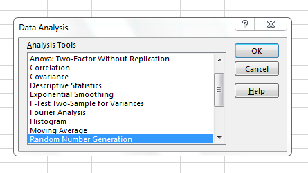
Upon clicking the Data Analysis button, a pop-up containing many statistical tools are available. Locate Random Number Generation as seen in Figure 3.16 and click ok. You should obtain another pop-up that looks similar to Figure 3.17.

Figure 3.17: Random Number Generation Menu

We can use the random number generation tool to also create a sample of random data. In the following example, we will use the random number generation applet to construct a random sample from a weighted dice.

Example 3.1.7.

Let’s create a random sample of 200 dice rolls involving 2 dice with the following weights:

Side:	1	2	3	4	5	6
Weights:	0.4	0.2	0.2	0.05	0.05	0.1

Note that the weights determine the how likely that side will arise. That is, the value of 1 will show up more than 4 or 5 since its weight is more.

In column $\tt{\color{red}\colorlet{pgfstrokecolor}{.}A}$ and $\tt{\color{red}\colorlet{pgfstrokecolor}{.}B}$ in Excel, create the same table column-wise. Figure 3.18 demonstrates this.

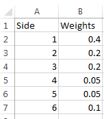
In cell $\tt{\color{red}\colorlet{pgfstrokecolor}{.}C1}$ and $\tt{\color{red}\colorlet{pgfstrokecolor}{.}D1}$ , type Dice 1 and Dice 2. We will generate our sample in these two columns.

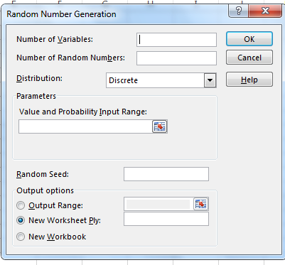
Open up the Random Number Generation tool. Propagate the empty input boxes according to Figure 3.19.

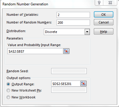
Figure 3.19: Random Number Generation Filled-In

Since we have 2 dice, then there are 2 variables. We want to generate 200 random numbers for each of the variables. Since our variables are discrete in nature, we have selected this for the distribution entry. Either use the button to select the appropriate range stated in Figure 3.19 or manually type the range as stated for the Value and Probability Input Range and Output Range. These will inform Excel what the values/weights are and where they should be outputted within the spreadsheet.

Figure 3.20: Portion of Weighted Dice Sample

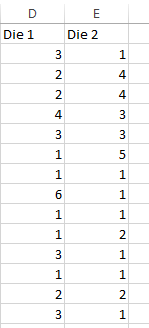
After clicking OK, the sample for the dice is generated, as seen in Figure 3.20 $\clubsuit$

There are many additional tools that Excel is capable of doing. This section is not intended to demonstrate all of Excel’s capabilities. For more shortcuts and techniques in Excel, we refer the reader to [] and references therein. If there are any additional tools and techniques in Excel that are needed for explaining concepts, we will demonstrate them appropriately.

Concepts Check: 1. Evaluate the expression

\frac{2e^{-2}-\sqrt{3}}{4-(3-\sqrt{5})^{2}}

Answer:

-0.427753447

2. Recalculate the expression in Example 3.1.1 by changing the data in column

\tt{\color{red}\colorlet{pgfstrokecolor}{.}A}

2.0

2.2

2.4

2.6

, and

2.8

. Leave cell

\tt{\color{red}\colorlet{pgfstrokecolor}{.}B1}

as 2.4. Answer:

0.1

3. By manipulating

\tt{\color{red}\colorlet{pgfstrokecolor}{.}RAND()}

, create an expression which will randomly generate a value between -1 and 1. Answer:

\tt{\color{red}\colorlet{pgfstrokecolor}{.}=2*RAND()-1}

3.1.3 Exercises

1.
Answer each of the following statements as True or False.
1. (a)
  
  In order for Excel to compute mathematical expressions, the syntax must start with a $\tt{\color{red}\colorlet{pgfstrokecolor}{.}=}$ .
2. (b)
  
  The $\tt{\color{red}\colorlet{pgfstrokecolor}{.}\$}$ in mathematical expressions is used to only denote currency.
3. (c)
  
  Excel follows the order of operations that is taught in any algebra class.
4. (d)
  
  $\tt{\color{red}\colorlet{pgfstrokecolor}{.}RAND()}$ generates a random number between 0 and 2.
5. (e)
  
  $\tt{\color{red}\colorlet{pgfstrokecolor}{.}RANDBETWEEN(-1,1)}$ could output the value of 0.01.
2.
Compute the following expressions using Excel.
1. (a)
  
  $\sqrt{\dfrac{(2.4-4.467)^{2}+(1.2-4.467)^{2}+(9.8-4.467)^{2}}{2}}$
2. (b)
  
  $1+3.3\ln(200)$
3. (c)
  
  $\dfrac{1}{\sqrt{6\pi}}e^{-\frac{(2-4)^{2}}{6}}$
4. (d)
  
  $\dfrac{-(0.4)^{3}}{3\ln(1-0.4)}$
3.
Using Cell-Referencing in Excel, create functions which call cells to perform the following expressions. Note that $x_{1},x_{2},\ldots,x_{5}$ is meant to represent a continuous list of $5$ data points between $[0,1]$ . Do no try to simplify the expression.
1. (a)
  
  $\dfrac{50x_{1}+20x_{2}+15x_{3}+7x_{4}+8x_{5}}{100}$
2. (b)
  
  $\dfrac{2x_{1}+5x_{2}}{7}+\sqrt{\dfrac{(x_{3}-4)^{3}+(x_{4}-4)^{3}+(x_{5}-4)^{3% }}{8}}$
4.
Using Cell-Referencing, create functions which call cells to perform the following expressions. Note that $x_{1},x_{2},x_{3}$ is meant to represent a discrete list of $3$ data points between $[0,10]$ . Do not try to simplify the expression.
1. (a)
  
  $(x_{1}-\frac{1}{3}(x_{1}+x_{2}+x_{3}))+(x_{2}-\frac{1}{3}(x_{1}+x_{2}+x_{3}))+% (x_{3}-\frac{1}{3}(x_{1}+x_{2}+x_{3}))$
2. (b)
  
  $\ln(e^{x_{1}+x_{2}+x_{3}})-e^{\ln{(x_{1}+x_{2}+x_{3})}}$
5.

Qualitative Variables are those that are take on descriptive outputs. These variables may have numeric outputs, but arithmetic may not make sense. Examples of qualitative variables are shoe brands, addresses, favorite color, etc. We can use the random number generator concept to generate a random sample of data from qualitative variables. Develop a way to create a random sample of 200 of the qualitative variable SURVEY RESPONSES, with possible outputs: strongly disagree, diagree, neutral, agree, strongly agree. Note that each of the outputs are equally likely. (Hint: Uniform).
6.

Qualitative Variables can be further organized into two categories: ordinal and nominal. Qualitative ordinal variables are those that have descriptive outputs that can be put into a natural order (alphabetical doesn’t count). Qualitative nominal variables are those that have outputs that can’t be put into a natural order. In the previous example, what type of qualitative variable is SURVEY RESPONSES? Can you come up with a qualitative variable that is not the same type of qualitative variable as that of SURVEY RESPONSES?
7.

Generate a random sample of 20 data values that represent the the seconds on a clock. Is this a continuous variable or a discrete variable? What’s the population?