12.2 Paired Samples -test
| Goals: |
|
Referring to the introduction of this chapter, suppose that a physical therapist has developed a new treatment that she believes will improve flexibility for people suffering from rotator cuff injuries. How might she test the claim? A natural thing to do would be something akin to the following: Select a sample of people suffering from the same rotator cuff injuries. In a consistent fashion numerically measure flexibility of each subject. Then have each subject perform the treatment for the same amount of time. Once completed, using the same technique to measure flexibility, retest each subject. This generates two samples of numbers, but the samples are paired.
Suppose again that and are populations of numbers with means and respectively. The populations are paired if for each member in there is a corresponding member in and vice versa.
To execute a test on the two means, one needs samples from and If and are paired, the samples will be naturally paired. If the difference makes sense, then a Paired-Samples T-Test may be appropriate in testing the competing hypotheses.4747Populations can be paired, but taking a difference might be nonsensical. For example, if is the collection of all heights (in inches) of living Americans, and is the population of all weights (in pounds)of living Americans, then these populations are paired, but computing does not make sense.
It is important to be able to identify paired data, as treating paired data as unpaired weakens the analysis (knowledge of the samples would be discarded).
Example 12.2.1.
A researcher wished to test whether filling a football with air or helium would change the average distance of a punt. One set of footballs were filled with air and the other were filled with helium. Each football was punted by the researcher, and the distance recorded in yards. Are the samples paired or unpaired?
Solution. There is no relationship between the two samples of gas-filled footballs, so the data is unpaired.
Example 12.2.2.
A researcher wished to test whether consuming caffeine shortens the average time it takes to run a mile. To test the claim, she timed participants running a mile. One week later, allowing participants time to recuperate, she gave each participant a 29 mg caffeine tablet, and then ten minutes after consuming the tablet, she timed participants running another mile. Are the samples paired or unpaired?
Solution. For each subject two identical measurements are made, one before the treatment (caffeine given) and one after. Thus, the data is paired.
Suppose that and are paired populations of numbers where makes sense. For each pair of corresponding members and in and respectively, the difference makes sense as well. The population of differences consisting of all differences of pairs is well-defined and has mean
Thus, a hypothesis test on the difference of means is equivalent to a test on the mean If it is reasonable to assume the population is normally distributed4848If and are normally distributed, then is also normally distributed. or if the sample size taken from sufficiently large, then is is reasonable to use a -Test on the sample of differences.
Let’s set up notation for the test. The competing hypotheses will be one of the following three cases:
| direction of extreme | hypotheses | equivalent hypotheses |
|---|---|---|
| to the left | ||
| to the right | ||
| two-sided | ||
Suppose that from paired populations and paired samples of size are generated:
For each pair compute the difference The collection …, is then the samle of size from the population of differences The data can be summarized in a table such as this:
Let and denote the sample mean and sample standard deviation of the differences The test statistic is then
| (12.1) |
with
Example 12.2.3.
A researcher wished to test whether consuming caffeine shortens the average time it takes to run a mile. To test the claim, she timed participants running a mile. One week later, allowing participants time to recuperate, she gave each participant a 29 mg caffeine tablet, and then ten minutes after consuming the tablet, she timed participants running another mile. At a significance level of 10%, test whether the data below (running times are in minutes) provide significant evidence that consuming caffeine does lower the average time to run a mile. Assume that the differences in times are normally distributed.
Solution. Recall that if we let and denote the running time before and after consuming caffeine, respectively, and if we let then the competing hypotheses are
and the direction of extreme is to the left.
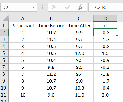
The first computation is to compute the differences of the pairs, using the order as given in the choice for This is shown in Figure 12.1.
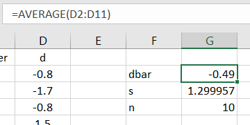
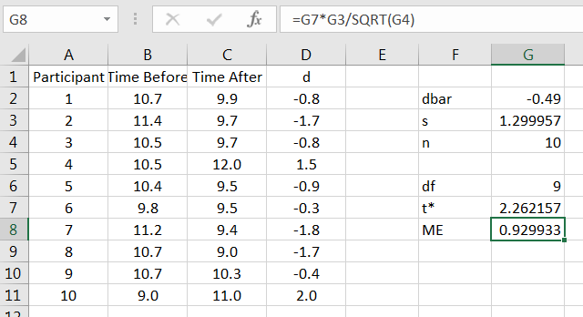
Then compute the summary statistics for the sample differences, as shown in Figure 12.2.
Lastly, compute the test statistic and -value, as in Figure 12.3.
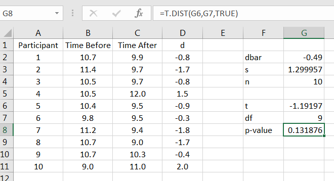
With and -value = 0.1319, at the significance level 10%, there is insufficient evidence that consumption of caffeine lowers the average running time of a mile.
Remark: As in Section LABEL:Sec:effect-size-single-mean, if the test yields a significant result, then it is appropriate to estimate the effect size using Cohen’s
12.2.1 Confidence Interval for Difference of Means - Paired Case
If the two samples are paired, and if it is reasonable to assume that the differences come from a normally distributed population, or if the number of pairs is sufficiently large, then a confidence interval on the difference of means can be constructed using a -Distribution as in Section 8.1.2:
| (12.2) |
Example 12.2.4.
A researcher wished to test whether consuming caffeine shortens the average time it takes to run a mile. To test the claim, she timed participants running a mile. One week later, allowing participants time to recuperate, she gave each participant a 29 mg caffeine tablet, and then ten minutes after consuming the tablet, she timed participants running another mile. Assuming the differences in times are normally distributed, use the sample data below to construct a 95% confidence interval for the difference of mean running times.
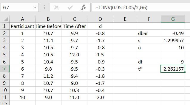
Solution. As with the hypothesis test, first compute the differences of the pairs, followed by the summary statistics for the sample of differences. Then, compute the the value of using the desired level of confidence, as in Figure 12.4.
Lastly, compute the upper and lower bounds for the confidence interval, as in Figure 12.6.
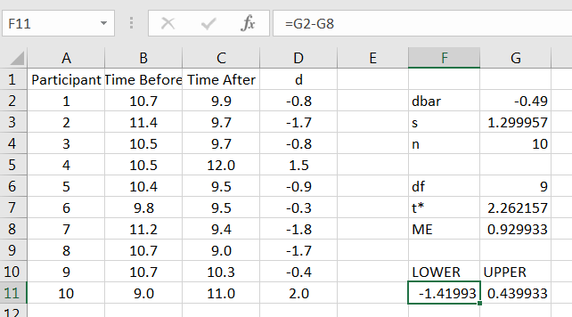
Thus, we are 95% confident that the true difference of mean running times is between -1.42 and 0.44 minutes.
12.2.2 Exercises
-
1.
A researcher thinks that a summer program for high school students would improve average interest in engineering as a profession. To test the claim, she measures participant interest in engineering before and after the summer program. Measurements are rankings of interest from 0 to 100, with larger values denoting greater interest. At a significance level of 5%, does the data below provide significant evidence that the summer program improves interest in engineering? You may assume that the population of differences is normally distributed.
-
(a)
What is the population of interest?
-
(b)
State the competing hypotheses.
-
(c)
What is the direction of extreme?
-
(d)
What test will you use, and why is it reasonable to use?
-
(e)
Compute the test statistic and corresponding -value.
-
(f)
Sketch the -value.
-
(g)
State your conclusion, i.e., do you reject or fail to reject
-
(h)
State the conclusion in a manner appropriate for a scientific journal.
-
(i)
What type of error could have been made?
-
(j)
Compute and interpret the effect size if the result is significant.
-
(a)
-
2.
Create a Python function called, paired_T_test that takes two sets of paired data and performs a paired samples -test. It should output the test statistic and the -value. In addition, based on the given, it should also output the decision.
-
3.
A researcher thinks that a summer program for high school students would improve average interest in engineering as a profession. To test the claim, she measures participant interest in engineering before and after the summer program. Measurements are rankings of interest from 0 to 100, with larger values denoting greater interest. Assuming that the population of differences is normally distributed, use the paired samples below to construct a 90% confidence interval for the true mean difference in change of interest in engineering as a profession. Interpret your results.