12 Testing Two Population Means 12.2 Paired Samples

T

12.3 Two Independent Samples $T$ -test

Goals:

\bullet

Learn how to identify independent samples;

\bullet

Learn how to do a Two Independent Samples

T

-test;

\bullet

Learn how to build a confidence interval using two

independent samples.

Suppose that $X$ and $Y$ are populations of numbers with means $\mu_{X}$ and $\mu_{Y},$ respectively, and suppose that the difference $\mu_{X}-\mu_{Y}$ makes sense. Suppose further that we wish to make a decision on the difference $\mu_{X}-\mu_{Y},$ but that in doing so, the samples drawn from $X$ and $Y$ are independent, i.e., selections from $X$ have no impact on selections from $Y .$ In this situation, it may be appropriate to perform a Two-Independent Samples $T$ -Test, which we introduce in this section.

Suppose that $x_{1},x_{2},\ldots,x_{m}$ is a simple random sample drawn from $X,$ and $y_{1},y_{2}\ldots,y_{n}$ is a simple random sample independently drawn from $Y .$ If the populations $X$ and $Y$ are normally distributed, or if the sample sizes $m$ and $n$ are both sufficiently large, then it is reasonable to use a $T$ -Test with test statistic given by

t=\frac{(\bar{x}-\bar{y})-(\mu_{X}-\mu_{Y})}{\sqrt{\frac{s_{x}^{2}}{m}+\frac{s% _{y}^{2}}{n}}},\qquad df=\mbox{smaller of }m-1\mbox{ and }n-1.

(12.3)

If it is reasonable to assume that the populations $X$ and $Y$ have equal variances, then the test statistic reduces to

t=\frac{(\bar{x}-\bar{y})-(\mu_{X}-\mu_{Y})}{s_{p}\sqrt{\frac{1}{m}+\frac{1}{n% }}},\qquad df=m+n-2,

(12.4)

where $s_{p}$ denotes a pooled standard deviation and is given by

s_{p}=\sqrt{\frac{(m-1)s_{x}^{2}+(n-1)s_{y}^{2}}{m+n-2}}.

(12.5)

If you are unsure whether it proper to assume that $X$ and $Y$ have the same variance, then use Equation (12.3). But, if you can assume the variances are the same, then Equation (12.4) is preferred.⁴⁹⁴⁹Assuming the variances are equal is additional information, meaning a likely stronger result. The pooled standard deviation probably won’t change the value of $t$ by much, but the larger degrees of freedom will likely yield a smaller $p$ -value.

Example 12.3.1.

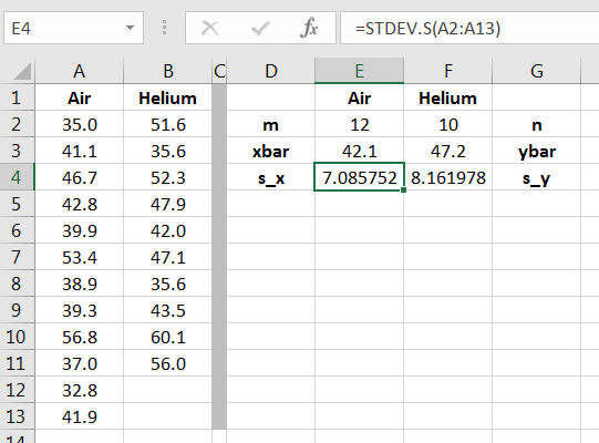
A researcher wished to test whether filling a football with air or helium would change the average distance of a punt. One set of footballs were filled with air and the other were filled with helium. Each football was punted by the researcher, and the distance recorded in yards. The data is given in the table below. At a significance level of 5%, determine whether there is significant evidence that the true average distance of helium-filled punts is different from the true average distance of air-filled punts. Assume that the two populations of distances are normally distributed.

\begin{array}[]{c|c}\mbox{\bf Air}&\mbox{\bf Helium}\\ \hline 35.0&51.6\\ 41.1&35.6\\ 46.7&52.3\\ 42.8&47.9\\ 39.9&42.0\\ 53.4&47.1\\ 38.9&35.6\\ 39.3&43.5\\ 56.8&60.1\\ 37.0&56.0\\ 32.8&\\ 41.9&\\ \end{array}

Solution. Recall that if we let $\mu_{a}$ and $\mu_{h}$ denote the true averages of the researcher punting distances of air-filled and helium-filled footballs, respectively, then the competing hypotheses are:

\begin{array}[]{ll}H_{0}:&\mu_{a}-\mu_{h}=0\\ H_{1}:&\mu_{a}-\mu_{h}\neq 0\\ \end{array}

The direction of extreme is two-sided, and the samples are independent. Since the populations are normally distributed, a two-independent samples $T$ -Test is appropriate. One way to assess if it is reasonable to assume the population standard deviations are equal is to examine the summary statistics, as shown in Figure 12.7.

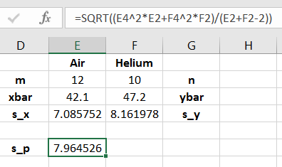
We will add to a repertoire of assessing when two standard deviations are not the same, but $s_{x}=7.09$ and $s_{y}=8.16$ do not strongly suggest different variances, so we will use the pooled test. The computation of $s_{p}$ using Equation (12.5) is shown in Figure 12.8.⁵⁰⁵⁰Make a note that what you get is between $s_{x}$ and $s_{y}.$ If it isn’t, then something went wrong in the calculation.

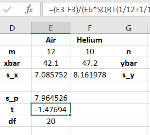
Figure 12.8: Pooled Sample Standard Deviation

Now use Equation (12.4) to compute the test statistic, as in Figure 12.9.

Recalling that this is a two-sided test, the $p$ -value calculation is shown in 12.10.

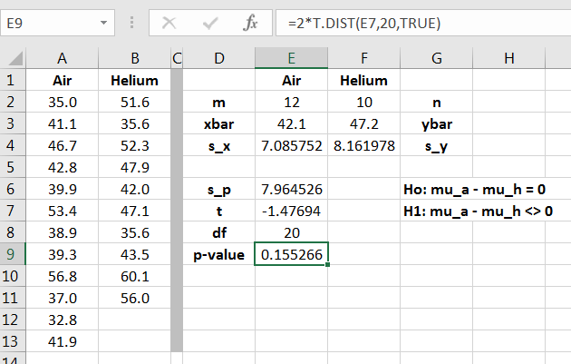
Since the $p$ -value is greater than 0.05, we fail to reject $H_{0}.$ That is, there is insufficient evidence that the true average punting distances (when kicked by the researcher) are different whether the football is filled with air or helium.

$\clubsuit$

Example 12.3.2.

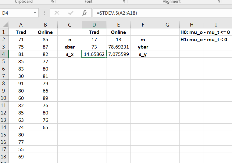
A study was conducted to assess whether student learning in college algebra would improve in an online course versus a traditional classroom. A single instructor with experience in both environments was selected to run two courses, one traditional and one online. A group of 50 college algebra students were randomly assigned to either of the two sections, so that 25 were in each. At the end of the semester, students were given a common final exam. The scores on the final are given below. Using the data, at a 10% significance level, determine if there is significant evidence that student learning is improved in online college algebra courses. Assume that the two populations of final exam scores are normally distributed.

\begin{array}[]{c|ccccccccccccccccc}\mbox{\bf Trad}&71&75&81&85&83&30&91&80&60% &82&85&63&74&80&77&55&69\\ \hline\mbox{\bf Online}&85&87&82&77&80&81&79&66&89&76&80&76&65\\ \end{array}

Solution. Let $\mu_{o}$ and $\mu_{t}$ denote the true average exam score for online and traditional college algebra courses taught by the instructor, respectively. The competing hypotheses are:

\begin{array}[]{ll}H_{0}:&\mu_{o}-\mu_{t}\leq 0\\ H_{1}:&\mu_{o}-\mu_{t}>0\\ \end{array}

The direction of extreme is to the right.

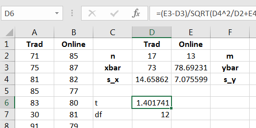
By computing the summary statistics as in Figure 12.11, it is evident that assuming the population variances are the same is not reasonable.

Using Equation (12.3), the test statistic is shown in Figure 12.12.

The $p$ -value is given in Figure 12.13.

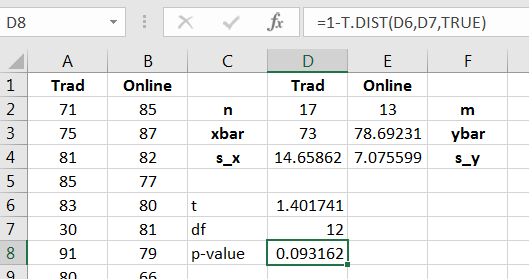
Since the $p$ -value is not larger than 0.1, we reject $H_{0},$ i.e., there is significant evidence that the true average exam score in the online courses is larger than the true average score in the traditional courses. $\clubsuit$

12.3.1 Confidence Interval for a Difference of Means - Independent Case

We can construct confidence intervals for the difference of two means using the $T$ -distribution, assuming the proper assumptions hold first. That is, if the two samples come from normal distributions or if the sample sizes are sufficiently large. For the independent case, we must know whether or not the samples come from random variables with same variances. This, again, will determine whether we use Eq. (12.3) or Eq. (12.4).

Let’s first look at the case when the the samples come from random variables with different variances. In this case, the confidence interval would be constructed based on the following formula.

(\bar{x}-\bar{y})\pm t^{*}\sqrt{\frac{s_{x}^{2}}{m}+\frac{s_{y}^{2}}{n}}

(12.6)

The degrees of freedom is then given by the smaller of $m-1$ or $n-1$ .

Example 12.3.3.

A study was conducted to assess whether student learning in college algebra would improve in an online course versus a traditional classroom. A single instructor with experience in both environments was selected to run two courses, one traditional and one online. A group of 50 college algebra students were randomly assigned to either of the two sections, so that 25 were in each. At the end of the semester, students were given a common final exam. The scores on the final are given below. Assume that the two populations of final exam scores are normally distributed. Construct at 98% confidence interval for the difference in mean exam scores.

\begin{array}[]{c|ccccccccccccccccc}\mbox{\bf Trad}&71&75&81&85&83&30&91&80&60% &82&85&63&74&80&77&55&69\\ \hline\mbox{\bf Online}&85&87&82&77&80&81&79&66&89&76&80&76&65\\ \end{array}

Solution. Extracting all of the pertinent descriptive stats we have the following.

After obtaining the test statistic $t^{*}$ and the $M E$ , we plug the respective values into Eq. (12.3).

$\clubsuit$

For the case when we can assume equal variances, we instead calculate the pooled variance, $s_{p}$ . This used Eq. (12.5). Thus, the confidence interval formula is given as

(\bar{x}-\bar{y})\pm t^{*}s_{p}\sqrt{\frac{1}{m}+\frac{1}{n}},

(12.7)

with $df=m+n-2$ .

Example 12.3.4.

A researcher wished to test whether filling a football with air or helium would change the average distance of a punt. One set of footballs were filled with air and the other were filled with helium. Each football was punted by the researcher, and the distance recorded in yards. Assume that the two populations of distances are normally distributed and that their variances are equal. Construct an 85% confidence interval for the difference in distance kicked.

\begin{array}[]{c|c}\mbox{\bf Air}&\mbox{\bf Helium}\\ \hline 35.0&51.6\\ 41.1&35.6\\ 46.7&52.3\\ 42.8&47.9\\ 39.9&42.0\\ 53.4&47.1\\ 38.9&35.6\\ 39.3&43.5\\ 56.8&60.1\\ 37.0&56.0\\ 32.8&\\ 41.9&\\ \end{array}

Solution. Extracting all of the pertinent descriptive stats we have the following.

Calculating the poolled standard deviation, the test statistic, and the mean error, we can plug in the values into Eq. (12.4).

$\clubsuit$

12.3.2 Exercises

An engineer is interested if a new sheet metal molding machine performs faster than an older version a company has been using. In order to test this claim, the times to complete the same mold are recorded for both the new machine and for the old machine. Below are their times in seconds. The data is assumed to come from normally distributed random variables. Assume that the variances are equal. Answer the following.

Old	32.73	33.32	33.83	32.27	33.39	33.11	31.70	33.82	32.67	32.62
New	30.72	30.86	31.84	31.58	31.90	33.02	31.34	30.63	32.12	30.76

(a)

What is the population of interest?
(b)

State the competing hypotheses.
(c)

What is the direction of extreme?
(d)

What test will you use, and why is it reasonable to use?
(e)

Compute the test statistic and corresponding $p$ -value.
(f)

Sketch the $p$ -value.
(g)

Using $\alpha=0.05$ , state your conclusion, i.e., do you reject $H_{0}$ , or fail to reject $H_{0}$ ?
(h)

State the conclusion in a appropriate for a scientific journal.
(i)

What type of error could have been made?
(j)

Calculate a 95% confidence interval for the difference in means.

2.
Differences in post-test/pre-test scores are calculated in an effort to determine if curriculum changes are beneficial. Suppose two groups receive the same instruction except for one extra unit is taught to Group B. Group A does not receive this instruction. Both groups received the same exams regardless if they knew the material or not. Below is a sample taken between the groups. Assume the data comes from normally distributed random variables and that variances are not equal.

Group A -1 -1 -3 -3 1 0 2 4 3 2

Group B -1 1 0 2 2 1 1 1 0 1
1. (a)
  
  What is the population of interest?
2. (b)
  
  State the competing hypotheses.
3. (c)
  
  What is the direction of extreme?
4. (d)
  
  What test will you use, and why is it reasonable to use?
5. (e)
  
  Compute the test statistic and corresponding $p$ -value.
6. (f)
  
  Sketch the $p$ -value.
7. (g)
  
  Using $\alpha=0.05$ , state your conclusion, i.e., do you reject $H_{0}$ , or fail to reject $H_{0}$ ?
8. (h)
  
  State the conclusion in a appropriate for a scientific journal.
9. (i)
  
  What type of error could have been made?
10. (j)
  
  Calculate a 95% confidence interval for the difference in means.

12.3 Two Independent Samples T-test

Example 12.3.1.

Example 12.3.2.

12.3.1 Confidence Interval for a Difference of Means - Independent Case

Example 12.3.3.

Example 12.3.4.

12.3.2 Exercises

12.3 Two Independent Samples $T$ -test