10 Testing a Single Population Mean 10.6 Optional: Effect Size 10.8 Python Commands for Testing a Single Mean

10.7 Confidence Intervals and Two-Sided Hypothesis Tests

A two-sided test on a population mean $\mu$ can be conducted using a confidence interval for $\mu.$ We’ll use a $T$ -Test to illustrate.

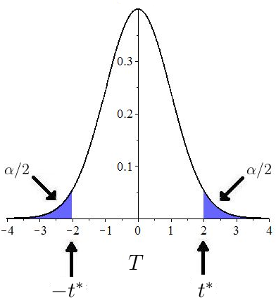
Suppose that the null hypothesis is $H_{0}:\mu=\mu_{0},$ and suppose that the significance level for the test is $\alpha.$ Recall that the rejection region for a hypothesis test is the collection of values for the test statistic in which the null hypothesis is rejected. Let $t^{*}$ denote the critical value, i.e., the value that bounds the critical region as shown in Figure 10.38.

The critical value, $t^{*}$ , is the same value of $T$ used in constructing a $(1-\alpha)\cdot 100\%$ confidence interval,

\bar{x}\pm t^{*}\frac{s}{n},

where $n,$ $\bar{x},$ and $s$ are summary statistics for a sample. Now the test statistic for the sample is

t_{0}=\frac{\bar{x}-\mu_{0}}{s/\sqrt{n}},

and $H_{0}$ is not rejected if $-t^{*}<t_{0}<t^{*}.$ This is equivalent to not rejecting $H_{0}$ if $\mu_{0}$ is in confidence interval, i.e.,

\bar{x}-t^{*}\frac{s}{n}<\mu_{0}<\bar{x}+t^{*}\frac{s}{n}.

The upshot, then, is that the null hypothesis is rejected precisely when the value $\mu_{0}$ does not land in the confidence interval.

Two examples will illustrate.

Example 10.7.1.

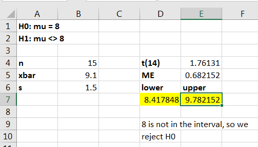
Suppose that $H_{0}:\mu=8$ is to be tested at the 10% level. Suppose that a simple random sample yields the summary statistics $n=15,$ $\bar{x}=9.1,$ $s=1.5,$ and assume that it is reasonable to assume that the sample came from a normally distributed population.

Now $t^{*}$ is chosen so that we are 90% confident that the true mean is in the confidence interval. Since $df=14,$ we want the area to the left of $t^{*}$ under the curve $T(14)$ to be 0.95. So,

t^{*}=\tt{\color{red}\colorlet{pgfstrokecolor}{.}T.INV(0.95,14)}\approx 1.76.

The margin of error for the confidence interval is

t^{*}\frac{s}{\sqrt{n}}=1.76\frac{1.5}{\sqrt{15}}\approx 0.68,

and so the 90% confidence interval is $9.1\pm 0.68,$ or in interval notation $(8.42,9.78).$ Since the interval does not contain $\mu_{0}=8,$ we reject $H_{0},$ i.e., there is significant evidence against $H_{0}.$

The calculation is shown in Figure 10.39.

$\clubsuit$

Example 10.7.2.

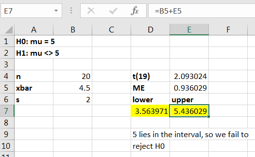
Suppose that $H_{0}:\mu=5$ is to be tested at the 5% level. Suppose that a simple random sample yields the summary statistics $n=20,$ $\bar{x}=4.5,$ $s=2.0,$ and assume that it is reasonable to assume that the sample came from a normally distributed population.

Now $t^{*}$ is chosen so that we are 95% confident that the true mean is in the interval. Since $df=19,$ we want the area to the left of $t^{*}$ under the curve $T(19)$ to be 0.975. So,

t^{*}=\tt{\color{red}\colorlet{pgfstrokecolor}{.}T.INV(0.975,19)}\approx 2.09.

The margin of error for the confidence interval is

t^{*}\frac{s}{\sqrt{n}}=2.09\frac{2.0}{\sqrt{20}}\approx 0.94,

and so the 95% confidence interval is $4.5\pm 0.94,$ or in interval notation $(3.56,5.44).$ Since the interval does contain $\mu_{0}=5,$ we would fail to reject $H_{0},$ i.e., there is insufficient evidence against $H_{0}.$

The calculation is shown in Figure 10.40.

$\clubsuit$

Concepts Check: 1. A hypothesis test is done on

H_{0}:\mu=25.

From a sample a confidence interval

(21.3,25.8)

is found. What decision is made? Answer: 25 is in the interval, so we fail to reject

H_{0}.

2. A hypothesis test is done on

H_{0}:\mu=12.

From a sample a confidence interval

(8.3,11.2)

is found. What decision is made? Answer: 12 is not in the interval, so we reject

H_{0}.

10.7.1 Exercises

1.

At a significance level of 5%, a hypothesis test is to be done on $H_{0}:\mu=20.$ A simple random sample of size 22 is taken, and a sample mean of 13.3 and sample standard deviation of 2.5 are found. Use a $T$ -Interval to make the decision.
2.

At a significance level of 10%, a hypothesis test is to be done on $H_{0}:\mu=30.$ A simple random sample of size 19 is taken, and a sample mean of 31.0 and sample standard deviation of 3.1 are found. Use a $T$ -Interval to make the decision.