10.2 Drug Manufacturing Example

Suppose we are running a pharmaceutical company that manufactures a commonly used drug, Drug U, that cures Illness A. For an adult with Illness A, a standard dosage of Drug U is a single 200 mg tablet every 8 hours. In the manufacturing process that produces 200 mg tablets of Drug U, there is inevitable variation in the actual weight of the pills as they are produced. It is important that the average weight of the tablets is very close to 200 mg, as dosage amounts too large or too small are bad for patients’ health.⁴⁰⁴⁰This implies too that the variance in tablet weights must be small, but that test is addressed in Chapter 11.

Manufacturing processes can go awry, needing periodic adjustments or more serious interventions. In this scenario, “going awry” translates to the mean weight, $\mu ,$ of pills being produced is different from 200 mg. This can be expressed in terms of two competing hypothesis:

Rejecting $H_0$ would result in halting manufacturing to correct whatever problems are necessary. Because halting manufacturing is costly, we don’t want to reject $H_0$ unless there is compelling evidence to do so.

Note that with an $H_0$ of $\mu =200,$ the direction of extreme is two-sided. That is, sample means larger (or smaller) than 200 mg give evidence against $H_0.$

Testing these hypotheses requires sample data. Before collecting data, the researcher should decide on the following:

1. 1.

   How the data will be analyzed, i.e., what statistical test(s) will be used. Doing this first helps ensure that good data are collected.⁴¹⁴¹Bad data are worthless.

2. 2.

   The significance level $\alpha .$⁴²⁴²Choosing $\alpha$ after computing a $p$-value is certainly unethical.

On the first decision, the following example will illustrate a common analysis. As for the second decision, though rejecting $H_0$ could be costly to the company, an unwillingness to reject $H_0$ could be dangerous to patients, so let’s choose $\alpha =\mathrm{0.05.}$

Suppose that a sample is generated, yielding the data given below:⁴³⁴³These data are given in the Excel file dutws.xlxs

Recall that the essential question in a hypothesis test is, “does the sample provide significant evidence against $H_0$?” To answer the question, we will compute a $p$-value based on the sample, and then compare that value to $\alpha .$

Using Excel, compute the summary statistics for the sample, as in Figure 10.1.

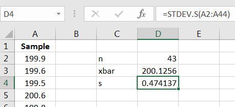
Note that $\overline{x}\approx 200.13$ is, indeed, not equal to 200, so this is evidence against $H_0.$ However, we are to judge whether this provides significant evidence against $H_0.$ This means that while this $\overline{x}$ looks close to 200, the difference of 0.13 must be judged relative to the population standard deviation $\sigma$ and sample size $n.$

Because the sample size $n=43$ is sufficiently large ($n\ge 30$), we can invoke the Central Limit Theorem and model the population of sample means $\overline{X}$ using a normal distribution with standard deviation $\sigma /\sqrt{n}.$ In symbols, we have

$$\overline{X}\sim N(\mu ,\frac{\sigma }{\sqrt{n}}),$$

and so the random variable

$$Z=\frac{\overline{X}-\mu }{\sigma /\sqrt{n}}$$

has a standard normal distribution, $N(0,1).$ If we knew $\sigma ,$ we would be able to compute the $p$-value, i.e., we could compute the chance of observing $\overline{x}=200.13,$ and anything more extreme, assuming $H_0$ is true.

Since, in manufacturing, a value for $\sigma$ is sometimes assumed to be known, let us suppose we are given that $\sigma =0.5$ mg.⁴⁴⁴⁴Two things: (1) It is not possible to know $\sigma$ without knowing $\mu ,$ but if a situation assumes a value for $\sigma ,$ then there are discipline-specific justifications, and (2) a $\sigma$ of 0.5 mg might be too large in this type of manufacturing process.

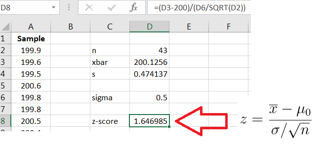
To calculate a $p$-value based on the observed $\overline{x},$ we compute the $z$-score for $\overline{x},$

$$z=\frac{\overline{x}-{\mu }_0}{\sigma /\sqrt{n}},$$

(10.1)

where ${\mu }_0$ is the hypothesized value of $\mu$ given in $H_0.$ In this example, the $z$-score is then

$$z=\frac{200.13-200}{0.5/\sqrt{43}}\approx 1.65,$$

as shown in Figure 10.2.

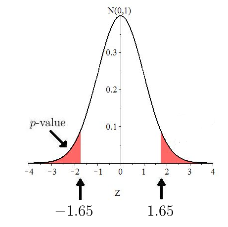
The calculation shows that the observed $\overline{x}$ is approximately 1.65 standard deviations above the mean, assuming $H_0$ is true. The $p$-value is the chance of observing $z=1.65,$ or anything more extreme, assuming $H_0$ is true. Now, because the direction of extreme is two-sided, ”anything more extreme” would be values $z\ge 1.65$ or $z\le -\mathrm{1.65.}$ The $p$-value is the shaded two-tailed region in Figure 10.3.

The $p$-value is twice the area to the right of 1.65, and we can compute that using Excel’s $\mathrm{𝙽𝙾𝚁𝙼}.\mathrm{𝙳𝙸𝚂𝚃}$. That is,

$$p\text{-value}=\mathrm{𝟸}*(\mathrm{𝟷}-\mathrm{𝙽𝙾𝚁𝙼}.\mathrm{𝙳𝙸𝚂𝚃}(\mathrm{𝙳𝟾},\mathrm{𝟶},\mathrm{𝟷},\mathrm{𝚃𝚁𝚄𝙴}))$$

gives the $p$-value, as shown in Figure 10.4. (Remember that $\mathrm{𝙽𝙾𝚁𝙼}.\mathrm{𝙳𝙸𝚂𝚃}$ gives area to the left, so subtract from 1 if you want area to the right.)

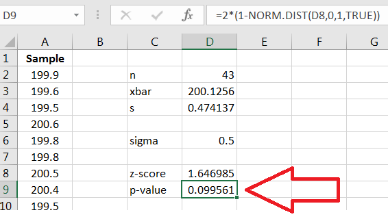
Since the $p$-value is $>\alpha ,$ we would fail to reject $H_0,$ that is, there is insufficient evidence that the manufacturing process is producing tablets of average weight different from 200 mg.

In failing to reject $H_0,$ a Type II error could have been made. But, recall that it is generally impossible to know whether the error has occurred. The probability that a Type II error has occurred is either 0 or 1: It is 1 if the error did occur, or it is 0 if the error did not occur.

Remarks: • This example illustrates a $Z$-test on a single population mean. Test on means are called parametric tests, as the test is done on a parameter of a population. Tests on population standard deviations and population proportions are also parametric tests. • In doing a test on a population mean, one should explore the sample data more than simply computing the summary statistics of $n,$ $\overline{x}$ and $s.$ Unless the sample is too small (e.g., $n=6$), at minimum a histogram of the sample data should be studied to assess if the test is appropriate. More on this later.