10.10 Optional: Robustness of the $T$-Test

Suppose $X$ is a population of numbers with mean $\mu .$ Because of the Central Limit Theorem, the $T$-Test is reliable regardless of the distribution of $X,$ as long as the samples are simple random and sufficiently large. We have the skills to simulate this with ease.

For example, suppose that $X$ has a uniform distribution from 0 to 20, so $X$ has a distribution quite different from normal. We know that $X$ has mean $\mu =10.$ Let’s run 1000 $T$-Tests on $H_0:\mu =10$ with a significance level $\alpha =\mathrm{0.05.}$ This is an abuse of the $T$-Test. as $X$ is not normal, but if the sample size is large enough, we should see about 5% Type I errors. Since we’ve been using $n\ge 30$ as a rule-of-thumb for “large enough,” let’s use samples of size 30 in the simulation.

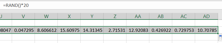
In Excel cell $\mathrm{𝙰𝟸}$ execute $=\mathrm{𝚁𝙰𝙽𝙳}()*\mathrm{𝟸𝟶}$. This will generate a random number from the population. (Recall that $\mathrm{𝚁𝙰𝙽𝙳}$ generates random numbers uniformly between 0 and 1.) Drag the command across to cell $\mathrm{𝙰𝙳𝟸}$, thus generating a random sample of size 30 from $X$ in row $\mathrm{𝟸}$, as shown in Figure 10.48.

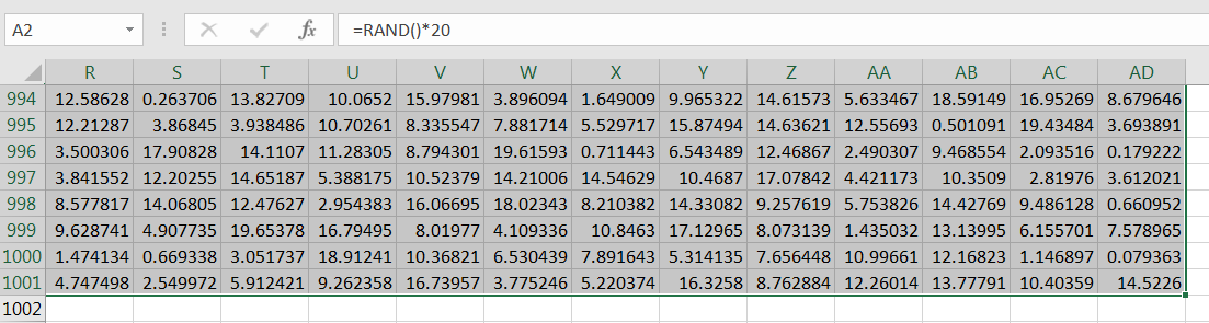
Now drag that row of commands down to row $\mathrm{𝟷𝟶𝟶𝟷}$ to create 999 more samples of size 30, as in Figure 10.49. (If you want to create more random samples than 1000, go for it.)

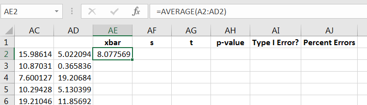
Compute the sample average for the first sample, as in Figure 10.50.

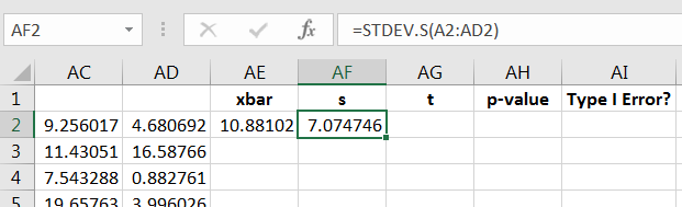
Similarly, compute the sample standard deviation for the first sample, as shown in Figure 10.51.

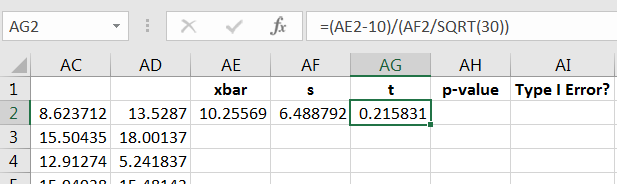
Since $X$ isn’t normally distributed, computing

won’t be a proper $t$-score, so label the column as you see fit, and then calculate Equation (10.9) for the first sample, as in Figure 10.52.

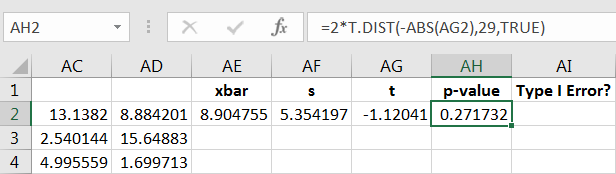
Since Equation (10.9) isn’t a true $t$-score, then using $𝚃.\mathrm{𝙳𝙸𝚂𝚃}$ isn’t a proper $p$-value calculation, so label that column as you see fit. Some “$t$”-scores will be positive and some negative, so we can calculate the “$p$”-value using the absolute value command as follows:

The calculation is shown in Figure 10.53.

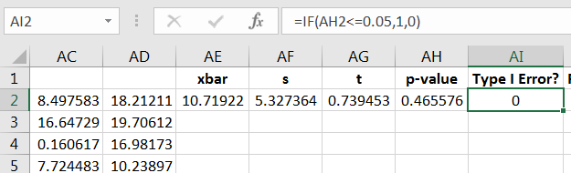
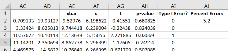
It the $p$-value is less than or equal to $\alpha ,$ then a Type I error will have occurred (we know $H_0$ is true). We can use the $\mathrm{𝙸𝙵}$ command to encode the result, with 0 denoting a correct decision, and 1 otherwise, as in Figure 10.54.

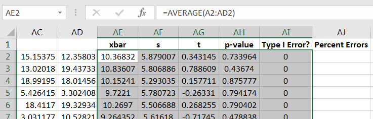
Now drag the four commands down to repeat the computations for the other 999 samples, as in Figure 10.55.

At last, compute the percent of Type I errors committed. This can be done by adding up the 0’s and 1’s, and then computing the percent, as in Figure 10.56.

Because the $\mathrm{𝚁𝙰𝙽𝙳}$ command is re-executed with each change to the spreadsheet, you can experiment with seeing how the percent of Type I errors changes with repeated 1000 simulations. Note that the percent of errors stays near 5%, implying the $T$-Test can be used reliably on a uniform population if the sample size is at least 30.